J. Cent. South Univ. Technol. (2011) 18: 1726-1732

DOI: 10.1007/s11771-011-0894-0

Numerical simulation on melt flow with bubble stirring and temperature field in aluminum holding furnace

ZHANG Jia-qi(张家奇)^{1, 2}, ZHOU Nai-jun(周乃君)¹, ZHOU Shan-hong(周善红)^{1, 3}

1. School of Energy Science and Engineering, Central South University, Changsha 410083, China;

2. College of Aerospace and Material Engineering, National University of Defense Technology, Changsha 410073, China;

3. Shenyang Aluminum and Magnesium Engineering and Research Institute, Shenyang 110001, China

? Central South University Press and Springer-Verlag Berlin Heidelberg 2011

Key words:

aluminum holding furnace; porous brick; bubble agitation; computational fluid dynamic method；

1 Introduction

Bubble column has been widely used in chemical processes (steel refining, agitation by gas injection, fermentations, etc) due to its excellent mass/heat transfer characteristics, simple construction and low cost [1]. In practice, it introduces gas into the bath using sparger, e.g. nozzle, perforated plate, or porous plug [2]. It has been found that porous plugs, which produce finer bubbles, offer a greater gas-liquid interfacial area that helps to improve the heat/mass transfer [1], though this area depends largely on liquid properties as well [3].

A number of experimental studies have been carried out to investigate the bubble characteristics in the bubble column, e.g. bubble size, size distribution, and gas hold-up. In the previous experimental studies, bubble characteristics were obtained through photographic technique [3] or electroresistivity probe [4]. KOIDE et al [5] measured the size of bubbles generated from porous plate, and they correlated the mean bubble size to the dimensionless numbers. This correlation was extended by IGUCHI et al [6], who investigated experimentally the effects of porous plug properties on the characteristics of bubbles generated through porous nozzle. POHORECKI et al [7] carried out a numerical experiment to correlate the mean bubble size to the liquid physical properties as well as superficial gas velocity; however, the effects of nozzle types were not involved.

Because of the inherent complexity of bubble column, computational fluid dynamic (CFD) method was more widely used for improving the design and optimizing the operating parameters. In general, two approaches are mostly used to simulate the multiphase flow in bubble column: the Euler-Euler approach and the Euler-Lagrange approach. The former one considers the dynamics of the dispersed phase ensemble averaged, thus the computational demands are much lower compared with Euler-Lagrange approach [8-10]. The latter one, which solves the emotional equations for every bubble, is more suitable for fundamental investigations [11-13].

To the best knowledge of the authors, there were not much published researches focusing on melt flow driven by porous plug bubbles in aluminum casting furnace. However, from the view of modeling, it can be seen as a bubble column flow. In the present study, Euler- Lagrange, more accurate under low discrete phase fraction [14], was used to simulate the melt flow driven by bubbles generated from porous brick.

2 Computational models

2.1 Geometrical model

Under the reference operating condition (ROC), the geometry of melt zone is illustrated in detail as shown in Fig.1. The geometrical model was built up consistent to the real size of the furnace, where the walls surrounding the melt would be excluded from the physical model and would be represented by boundary conditions instead.

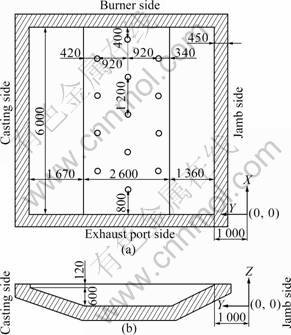
Fig.1 Physical model size and coordinate of melt zone: (a) X-Y plain section; (b) Y-Z plain section

2.2 Mathematical model

In Euler-Lagrange model, the conservation equations of continuous phase can be given by

                               (1)

               (2)

                    (3)

              (4)

                              (5)

Here, Eqs.(1), (2) and (3) represent mass, momentum and energy conservation, respectively. Equations (4) and (5) stand for the standard κ-ε model expressions describing the conservations of the turbulent kinetic energy κ and its dissipation rate. ρ_L is the density of molten aluminum, kg/m³. u_L is the velocity vector of liquid, m/s; t is the time, s. P is the pressure, Pa; g is the gravity acceleration, m/s². M is the momentum term caused by discrete phase, kg/m². τ_eff is the effective stress tensor,

where μ_L is the liquid viscosity, 0.001 1 kg/(m·s); μ_t is the turbulent viscosity, μ_t=c_μ·ρ·κ²ε^-1, and in the present turbulent model, c_μ is the empirical constant, 0.09; I is the unit tensor. h is the enthalpy, J/m³; h_p is the discrete phase enthalpy, J/m³. J_p is the diffusion rate of discrete phase, kg/(m²·s). k_eff is the effective thermal conductivity, k_eff=k_L+k_t, W/(m·K); k_L is the heat conductivity of liquid; k_t is the turbulent heat conductivity, k_t=C_pL·μ_t·Pr_t^-1; C_pL is the specific heat of melt, J/(kg·K); Pr_t is the empirical turbulent Prandtl number, 0.5. T is the temperature, K. κ is the turbulent kinetic energy, m²/s²; ε is the turbulent kinetic energy dissipation rate, m²/s³.   is the turbulent kinetic energy generation. Other empirical constants in the present turbulent model are listed as Pr_κ=1.0, Pr_ε,=1.3, C_ε1=1.44 and C_ε2=1.92.

The force acting on discrete phase (bubble) could be written as

               (6)

where u_p is the velocity vector of particle; ρ_p is the particle density, kg/m³; drag force F_D could be expressed as

                                 (7)

F represents other acceleration term acting on discrete phase including:

1) Virtual mass force

                            (8)

2) Force caused by pressure gradient

                               (9)

2.3 Initial and boundary conditions

2.3.1 Bubble size

Coalescence and break-up behaviors of the bubbles cannot be avoided during bubble rising in the liquid; thus the initial bubble size distribution may be changed during the upward motion of bubbles [15]. The previous investigation [1] classified the pattern of fine bubble driven flow into three regimes depending on gas flow rate: homogeneous bubbly flow, incipient coalescence bubbly flow and heterogeneous bubbly flow. The transition superficial velocities between these regimes were found to be intensively related to liquid and gas properties according to the previous studies. IGUCHI [6] proposed that if bubbles are very small and Re (=d_p·u_p·(ρ_L-ρ_p)·μ_L^-1, where d_p is the bubble diameter, m) is much smaller than 300, the bubbles would rise as discrete pattern without coalescence and disintegration.

GRACE [16] measured the terminal velocity of bubble rising in infinite Newtonian liquids and correlated Re versus Eo (=(ρ_L-ρ_p)·g·d_p²·σ_L^-1) for different Mo (=g·μ_L⁴·(ρ_L-ρ_p)^-1·σ_L^-3). Considering the bubble size, 0.2- 1.0 mm (according to the manual from manufacturer) and the physical properties of the melt, Mo number can be estimated to be 0.99×10^-14. Thus, the correlation between Re and Eo can be plotted in Fig.2 [16]. Further, we can evaluate that Eo ranges from 0.001 to 0.027, and the corresponding Re is much lower than 300 as Fig.2 shows. Thus, the break-up and coalescence phenomena of the bubbles can be ignored in the present study.

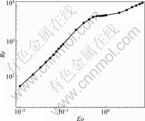
Fig.2 Correlation of Re versus Eo as Mo=0.99×10^-14 [16]

KOIDE et al [5] proposed the following empirical equation for evaluating the mean size of bubbles generated from a porous plug in homogeneous bubbly flow regime:

                (10)

where  is the mean bubble diameter, m; σ_L is the continuous phase-gas surface tension, 0.85 kg/s² for the present gas-liquid couple; d_pm is the pore diameter of porous sparger, m. Equation (10) shows that the mean bubble size increases with the increase of liquid-gas surface tension, gas superficial velocity and pore diameter; however, it decreases with the increase of liquid density. Unfortunately, Eq.(10) does not consider the effect of viscosity. However, the liquid viscosity seems to influence significantly the mean bubble size according to MOUZA et al’s finding [1], where a conclusion that the mean bubble diameter increases with the increase of liquid viscosity was confirmed. They also observed a narrow small bubble (<1 mm) distribution in aqueous alcohol solution with low viscosity (around 0.001 kg/(m?s)).

The previous studies have not given exact conclusion about the effect of bubble size on the flow field. Thus, in the present model, this sort of effect will be evaluated. Basically, the bubble size was assumed to be obedient to the Rosin-Rammler distribution from 0.2 to 1.0 mm with the mean size of 0.6 mm.

2.3.2 Bottom, side and top boundary

In the present numerical model, 13 porous bricks were represented by area elements, through which the bubbles were injected as inert particles. On these boundaries, a mass flux of 0.000 81 kg/s, i.e., a superficial velocity of 0.097 m/s, was designated.

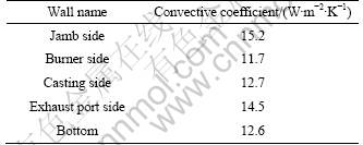
On the side and bottom boundaries of the melt zone, non-slip momentum boundary condition was enforced and thermal boundaries here were represented by “shell conduction”. Heat transfer coefficients from the outer side of the “shell” to ambient could be found in Table 1. By the way, reflections would happen once bubbles collide with the side walls.

Table 1 Heat transfer coefficient from outer wall of furnace to ambient [17]

Top boundary of the melt zone was set to be free surface, where a bubble would escape from the system once it touched the top boundary. Here, the heat supply from combustion chamber was represented by the boundary condition.

2.3.3 Initial conditions and calculation approach

Initially, the bulk melt was set to be quiescent and with the homogeneous temperature of 960 K. In addition, the solution domain was full of molten aluminum. In the numerical model, bubbles were ejected into the melt at t=0. Taking 1 h as the calculation period, the results represented the flow and thermal field of the melt after being heated and agitated for 1 h.

3 Results

3.1 Effect of bubble distribution on flow and thermal fields

Bubble size was set to be 0.2, 0.6, 1.0 mm, respectively, in the present numerical model, to examine the effect of bubble size on the flow and thermal fields. The results show that bubble size in the model has no significant effect on the melt flow and thermal fields.

3.2 Velocity field of melt

Figure 3 illustrates the melt velocity vectors obtained from numerical solution, and Fig.4 shows the melt velocity distribution. Obviously, on the top surface, the melt flows radially from the axis centers of the porous bricks to the edge sides. The farther from the porous bricks centers, the lower melt velocity can be found. In addition, on both the jamb side and casting side, the melt velocities are very low. These results all correspond with the phenomena observed.

Table 2 lists the max melt velocities on different horizontal sections. It is shown that on ROC, the vertical velocities of melt increase slightly from section Z=0.1 m to Z=0.5 m and decreases dramatically on section Z=  0.7 m. There are no significant differences among the horizontal velocity components in various sections, and the max horizontal velocity of the melt may be found on the melt top surface.

3.3 Temperature distribution in melt

Figure 5 shows the temperature distribution in the melt after being heated and agitated for 1 h. Apparently, the bulk melt temperature is quite even and the max temperature difference is less than 3 K in most area. The average temperature on the upper layer is higher than that on the lower layer slightly. Also, the highest temperature can be found within a thin layer of the melt surface, especially near the jamb side and casting side.

3.4 Melt temperature distribution during holding process

Holding process, without combustion or bubble induced, is also necessary to stratification and impurities separation for the melt. In this way without heating, some energy is lost from the top surface of the melt inevitably. In the present study, holding process was simulated based on a simplification that the top heat loss could be represented by a constant rate derived from systematic thermal measurement [17]. The numerical solution shows that, after 30 min holding, the max temperature variation increases from 10 to 60 K, as shown in Fig.6. Obviously, the closer to the top of the melt, the lower the temperature can be found, especially on the jamb side.

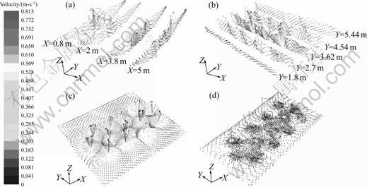
Fig.3 Velocity vectors on multiple sections in furnace: (a) Vertical to X; (b) Vertical to Y; (c) Z=0.7 m; (d) Z=0.1 m

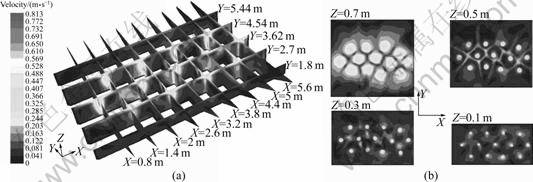
Fig.4 Melt velocity distributions: (a) Vertical sections; (b) Horizontal sections

Table 2 Max velocities on various horizontal sections

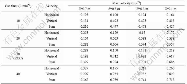
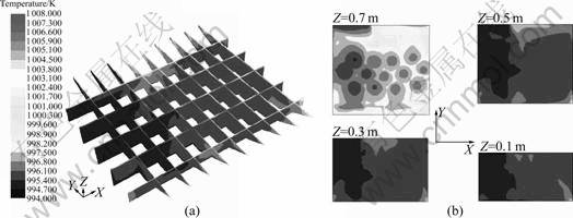
Fig.5 Melt temperature distribution: (a) Vertical sections; (b) Horizontal sections

4 Effect of gas flux on holding furnace performance

4.1 Holding furnace process

Molten aluminum with almost homogeneous temperature of 960 K would be induced into holding furnace from melting furnace where aluminum ingots are melted. Then, alloy materials will be added into the melt; simultaneously, the burner and gas suppliers start to work. This is known as the heating and agitation processing. According to the operating strategy, when the melt temperature reaches a certain value (usually 1 023 K), the combustion and argon flow cease, then the furnace just keeps holding for melt stratification. This is known as the holding process. During holding, the temperature of melt keeps decreasing. Once the melt temperature, which is measured by a thermocouple located at the center layer of the melt on the casting side, drops to a certain value preset, the burners and gas suppliers start to work again.

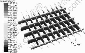
Fig.6 Melt temperature distribution after 30 min holding

4.2 Effect of gas flux on heating and agitation processing

The numerical solutions show that the gas flow rate does not affect the melt flow pattern. On the other hand, the effect of gas flow rate on the melt flow focuses on the velocity, as shown in Table 1. Obviously, the max melt velocities increase with the increase of gas flux. However, the increase rate of max velocities seems much lower than that of gas flux.

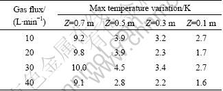
The effect of gas flux on the melt temperature distribution is obtained as well. Table 3 lists the max melt temperature difference on various horizontal sections, where no obvious differences can be found. In other words, the effect of gas flux on the homogeneity of melt temperature can be ignored.

Table 3 Maximum temperature variation on various horizontal sections

4.3 Effect of gas flux on melt temperature homogeni- zation after holding processing

After holding process, combustion and gas flow will start again. For evaluating the effect of gas flux on the melt temperature after holding process, and evaluating the utilization of gas flux on the alloying mixing, a couple of solutions were done by adopting the initial temperature condition, as shown in Fig.6. Figure 7 shows the max temperature difference in the melt versus the agitation duration for different gas fluxes.

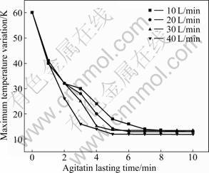
Fig.7 Max temperature variation versus agitation lasting time in different gas flux

Obviously, the curve representing 10 L/min shows that it takes as long as 10 min for the melt to recover the homogeneous temperature field, which demonstrates that the corresponding agitation intensity is very weak. The necessary duration to retrieve the homogeneous temperature field decreases to 6, 5, and 4 min as the gas flux increases to 20, 30 and 40 L/min, respectively. Thus, as the gas flux increases from 10 to 20 L/min, the stirring utilization likely shows a qualitative change. In fact, the major purposes of induced gas involve purifying the melt and accelerating the alloying process except homogenizing the melt temperature. Though there is no explicit correlation between the gas flux and utilization of melt mix or alloying, the effect of gas flux on the homogeneity of melt temperature can be taken as a reference.

4.4 Discussion

During the heating and agitation process, the numerical solutions show that the melt temperature keeps quite homogeneous anyway no matter lower or higher the gas flux is, and this is probably because the melt poured into the holding furnace is in almost homogeneous temperature. In addition, this may imply that the incline of metal loss is limited because of induced gas through porous bricks, as the metal oxidation increases exponentially with the temperature from 923 K upward [18].

A 30 min holding process causes a max temperature difference of 60 K in the bulk melt. The calculations show that after the holding process, the necessary duration for the stratified melt to recover the homogeneous temperature field is sensitive to the gas flux. This probably implies that the increase of gas flux enhances the corresponding effect on the alloying and degassing sensitively as well. However, obviously, a gas flux of 10 L/min seems too low to generate enough mixing on the melt alloying and degassing. With the increase of gas flux from 10 to 20, 30 and 40 L/min respectively, the necessary recovery time decreases from 10 to 6, 5 and 4 min, respectively. This implies that the agitation intensity increases gradually, and the alloying or degassing efficiency is also improved.

In fact, bubbles agitation plays key roles in the holding furnace process. Based on the results, the present study approves that, probably, good furnace performances (melt alloying, degassing) and lower argon usage may be reconciled. This depends on the process purpose. For instance, the gas flux can be kept lower if only homogeneous melt temperature is pursued; on the other hand, it has to be turned up for higher purification or alloying performance.

5 Conclusions

1) In the aluminum holding furnace, the coalescence and disintegration of bubbles can be ignored.

2) For the given furnace, the bubble size distribution does not affect flow and thermal field in the melt much.

3) As the melt poured into the holding furnace has almost homogeneous temperature, the gas flux does not affect the homogeneity of melt temperature much.

4) The gas flux of 10 L/min seems too low to generate enough mixing on the melt alloying or degassing.

5) According to the operation motive, the performance of melt alloying and degassing, and lower argon usage may be reconciled.

References

[1] Mouza A A, Dalakoglou G K, Paras S V. Effect of liquid properties on the performance of bubble column reactors with fine pore spargers [J]. Chem Eng Sci, 2005, 60: 1465-1475.

[2] Wang L, Lee H G, Hayes P. A new approach to molten steel refining using fine gas bubbles [J]. ISIJ Int, 1996, 36: 17-24.

[3] Camarasa E, Vial C, Poncin S, Wild G, Midoux N, Bouillard J. Influence of coalescence behaviour of the liquid and of gas sparging on hydrodynamics and bubble characteristics in a bubble column [J]. Chem Eng Process, 1999, 38: 329-344.

[4] Iguchi M, Kawabata H, Nakajima K, Morita Z I. Measurement of bubble characteristics in a molten iron bath at 1 600 ℃ using an electroresistivity probe [J]. Metall Mater Trans B, 1995, 26: 67-74.

[5] Koide K, Kato S, Tanaka Y. Bubbles generated from porous plug [J]. Chem Eng Jpn, 1968, 1: 51-56.

[6] Iguchi M, Kaji M, Morita Z. Effects of pore diameter, bath surface pressure, and nozzle diameter on the bubble formation from a porous nozzle [J]. Metall Mater Trans B, 1998, 29: 1209-1218.

[7] Pohorecki R, Moniuk W, Bielski P, Sobieszuk P, Babrowiecki G. Bubble diameter correlation via numerical experiment [J]. Chem Eng J, 2005, 113: 35-39.

[8] Pan Y, Dudukovic M P, Chang M. Dynamic simulation of bubbly flow in bubble columns [J]. Chem Eng Sci, 1999, 54: 2481-2489.

[9] Buwa V V, Ranade V V. Dynamics of gas-liquid flow in a rectangular bubble column: Experimental and single/multi-group CFD simulations [J]. Chem Eng Sci, 2002, 57: 4715-4736.

[10] Lahey R T, Drew D A. The analysis of two-phase flow and heat transfer using a multidimensional, four field, two-liquid model [J]. Nuc Eng Des, 2001, 204: 29-44.

[11] Laín S, Br?der D, Sommerfeld M, G?z M F. Modelling hydrodynamics and turbulence in a bubble column using the Euler-Lagrange procedure [J]. Int J Multiphase Flow, 2002, 28: 1381-1407.

[12] Buwa V V, Deo D S, Ranade V V. Eulerian-Lagrangian simulations of unsteady gas-liquid flows in bubble columns [J]. Int J Multiphase Flow, 2006, 32: 864-885.

[13] Deen N G, Solberg T, Hjertager B H. Large eddy simulation of the gas-liquid flow in a square cross-sectioned bubble column [J]. Chem Eng Sci, 2001, 56: 6341-6349.

[14] Mazumdar D, Guthrie R. A comparison of three mathematical modeling procedures for simulating fluid flow phenomena in bubble-stirred ladles [J]. Metall Mater Trans B, 1994, 25: 308-312.

[15] Alexiadis A, Gardin P, Domgin J F. Spot turbulence, breakup, and coalescence of bubbles released from a porous plug injector into a gas-stirred ladle [J]. Metall Mater Trans B, 2004, 35: 949-956.

[16] Grace J R. Shapes and velocities of bubbles rising in infinite liquids [J]. Chem Eng Res Des, 1973, 51: 116-120.

[17] Zhou Nai-jun. Report of systematic thermal measurement and analysis for melting and holding furnace [R]. Changsha: Central South University, 2008.

[18] Gamweger K, Bauer P. Energy savings and productivity increases at an aluminum slug plant due to bottom gas purging [C]// Neelameggham N R, Reddy R G, Belt C K, Vidal E E. Energy Technology Perspectives. Warrendale: TMS, 2009: 169-171.

(Edited by YANG Bing)

Foundation item: Project(2008AA11A116) supported by the National High Technology Research and Development Program of China

Received date: 2010-09-10; Accepted date: 2011-01-18

Corresponding author: ZHOU Nai-jun, Professor, PhD; Tel: +86-13973160806; E-mail: njzhou@mail.csu.edu.cn