

Regularized determination of interfacial heat transfer coefficient during ZL102 solidification process
SUI Da-shan(���ɽ), CUI Zhen-shan(����ɽ)
National Die and Mould CAD Engineering Research Center, Shanghai Jiao Tong University,
Shanghai 200030, China
Received 14 June 2007; accepted 23 August 2007
Abstract:
The interfacial heat transfer coefficient(IHTC) between the casting and the mould is essential to the numerical simulation as one of boundary conditions. A new inverse method was presented according to the Tikhonov regularization theory. A regularized functional was established and the regularization parameter was deduced. The functional was solved to determine the interfacial heat transfer coefficient by using the sensitivity coefficient and Newton-Raphson iteration method. The temperature measurement experiment was done to ZL102 sand mold casting, and the appropriate mathematical model of the IHTC was established. Moreover, the regularization method was used to determinate the IHTC. The results indicate that the regularization method is very efficient in overcoming the ill-posedness of the inverse heat conduction problem(IHCP), and ensuring the accuracy and stability of the solutions.
Key words:
solidification; regularization; inverse problem; parameter determination; sensitivity coefficient; interfacial heat transfer coefficient;
1 Introduction
The interfacial heat transfer coefficient(IHTC) between the casting and the mould is essential to the numerical simulation as one of boundary conditions. The inverse heat conduction method can be mainly used to determine the IHTC based on the temperature measurement data[1].
The inverse heat conduction problem belongs to the class of ill-posed problems, and its solution is sensitive to the temperature measurement data and it is difficult to satisfy the stability[2-3]. One of the earliest inverse methods was proposed to solve a quenching problem involving a spherical geometry[4-5]. BECK et al[1, 6] then introduced methods incorporating multiple future temperature measurements[1,6]. Subsequently, some researchers have used methods based on future time step and parameter-estimation methods proposed by BECK to solve a wide variety of inverse problems[7-9]. Many researchers have employed regularization method, dynamic programming, smoothing techniques, Kalman filtering, and conjugate gradient methods to solve the inverse heat conduction problems(IHCP)[10-18].
In this work, a new inverse method was presented according to the Tikhonov regularization theory. Moreover, a regularized functional was established to decrease the sensitivity of the temperature measurement data, overcome ill-posedness, and improve the accuracy and stability of the solution.
2 Mathematical model of DHCP
The direct heat conduction problem(DHCP) is to solve the temperature field when all material physical properties, and initial and boundary conditions are completely given in the casting process. The Fourier heat conduction equation can be solved to find the transient temperature field during casting solidification. This is a direct problem, and the mathematical model is as follows:
![]() (1)
(1)
The initial condition is
![]() (2)
(2)
The third boundary condition is
![]() (3)
(3)
where �� is density, �� is thermal conductivity, cp is specific heat, Q is heat resource, T0 is initial temperature, T1 and T2 are surface temperatures of casting and sand mold on the contact location respectively, and h is IHTC of the contact surface between casting and sand mold.
Various numerical methods can be used to solve the DHCP, such as the finite difference method(FDM), the boundary element method(BEM), and the finite element method(FEM). FEM was used to solve the transient temperature field of casting and sand mold during solidification in this work.
3 Mathematical model of IHCP
3.1 Tikhonov regularization mathematical model
The basic principle of the Tikhonov regularization method is to convert the ill-posed problem into a well-posed problem by adding a penalty term to the objective function.
In order to determine the IHTC, the functional was established according to the Tikhonov regularization theory[2-3]:
(4)

where ![]() represents the measured temperature at a certain time ti (i=1, ???, Nt) and well defined position xj (j=1, ???, Nm);
represents the measured temperature at a certain time ti (i=1, ???, Nt) and well defined position xj (j=1, ???, Nm); ![]() is the calculated temperature at time ti and position xj; h is the vector denoting all the unknown variables, and h={h1, h2, ???,
is the calculated temperature at time ti and position xj; h is the vector denoting all the unknown variables, and h={h1, h2, ???, ![]() }, where Nh is the number of unknown variables; ��T is an error of the measured temperature
}, where Nh is the number of unknown variables; ��T is an error of the measured temperature ![]() ��k is a typical interval within which each of the variable hk is allowed to vary around the initial value
��k is a typical interval within which each of the variable hk is allowed to vary around the initial value ![]() ; �� is the regularization parameter, and ����0.
; �� is the regularization parameter, and ����0.
The minimum of the functional J��(h) can be deduced to determine the unknown variable h. In order to minimize J��(h), there is
(5)

where Xijl is the sensitivity coefficient, and it can be expressed approximately as[7]

(6)
where ��hl is a priori perturbation of the variable hl, and the sensitivity coefficient can be calculated to investigate the variation of the response function, ![]() with ��hl.
with ��hl.
The Newton-Raphson iteration method was used to find the solution of Eqn.(5). There is
![]() (7)
(7)
where the increments ��hk can be solved by Taylor��s Formula and keeping only the linearization terms according to Eqn.(5).
It is defined as
(8)

![]()
(��lk is Kroneker operator) (9)
Then,
![]() (10)
(10)
3.2 Regularization parameter ��
There are two methods to determine the regularization parameter, i.e. a-priori method and a- posteriori method[3]. A-priori method was employed in this work.
According to Eqn.(4), it is defined as
![]() (11)
(11)
![]() (12)
(12)
Then,
![]() (13)
(13)
The regularization parameter can be evaluated by the following equation that deduced by referring to the illustration in Ref.[3] and considered the detailed feature of the inverse problem.
![]() (J��2(h)��0) (14)
(J��2(h)��0) (14)
3.3 Detailed iterative procedure of IHCP
The new inverse method can be implemented in a fairly simple way to determine the unknown variables. The iterative procedure is as follows.
1) At the beginning of the iterations, the components of vector h are initiated to some values, and the maximum number of iteration is defined.
2) The temperatures ![]() of the casting and sand mold are calculated with the direct FEM program.
of the casting and sand mold are calculated with the direct FEM program.
3) Each of the variable hk is varied by the priori perturbation ��hk and the temperatures are again calculated. The sensitivity coefficients are deduced by using Eqn.(6).
4) Using Eqns.(8), (9) and (10), the equations are solved to deduce the increment ��hk. If the maximum relative variation of the parameters is smaller than a desired tolerance, max|��hk/hk|����, then the iteration calculation will be finished. If not, the values, hk will be updated, ![]() and the calculation proceeds with the next iteration (step 2).
and the calculation proceeds with the next iteration (step 2).
4 Application of inverse method
Inverse analysis is performed to determine the IHTC for the aluminum alloy sand mold casting in the solidification process.
4.1 Temperature measurement experiment
Casting experiment was done to measure the temperature at different positions of the casting and sand mold, and the temperature measurement data were the input data of the IHCP to determine the IHTC.
Three-part molding was used in the casting experiment. The casting was aluminum alloy ZL102, and the sand mold was dry silicate bonded sand. Fig.1 shows the schematic diagram of casting process and the detailed structure dimension. The TC1, TC2, TC3 and TC4 are defined well the position of four thermocouples respectively. O point is supposed to be the coordinate origin, then the four positions�� coordinates are TC1(60.0,30.0), TC2(60.0,0.0), TC3(95.0,30.0) and TC4(100.0,30.0). The K type thermocouple was used to measure the temperatures, and the temperatures measure- ment data were recorded every 0.225 s.

Fig.1 Schematic diagram of casting process
The pouring temperature of aluminum alloy was 670.0 ��, and the initial temperature of sand mold was 30 ��. The temperature measurement curves at the four positions are illustrated in Fig.2. TC1M, TC2M, TC3M and TC4M denote the corresponding measured temperatures, respectively.
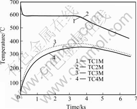
Fig.2 Temperature measurement curves of TC1, TC2, TC3 and TC4
4.2 Known conditions of numerical simulation
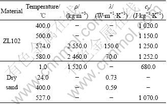
The physical properties of ZL102 and dry sand mold are the known conditions, and the nonlinear feature is considered to ensure the determination accuracy. The detailed values are listed in Table 1. The solidus temperature of ZL102 is TS=574.0 ��, the liquidus temperature is TL=580.0 ��, and the latent heat is L=480.0 kJ/kg. The equivalent specific heat method was used to calculate latent heat in numerical analysis. In addition, the convective heat transfer coefficient between sand mold and atmosphere is 35.0 W/(m2?K).
Table 1 Physical properties of ZL102 and dry sand mold
4.3 Mathematical model of IHTC
The main factor influencing IHTC is the temperature of casting and sand mold on the contact surface. Moreover, the thermal expansion coefficient of casting alloy is bigger by several orders of magnitude than that of sand mold. So the casting temperature is the most important influencing factor to IHTC. In the meantime other influencing factors are considered. Suppose IHTC is an exponential function of the temperature of casting surface, and the expression is defined as
![]() (hL��h0, TL��
(hL��h0, TL��![]() ) (15)
) (15)
where T is the temperature of casting surface, TL is liquidus temperature, ![]() is one temperature less than solidus temperature TS, and its value should be determined by the thermal expansion coefficient of casting and sand mold. It can be deduced that the temperature
is one temperature less than solidus temperature TS, and its value should be determined by the thermal expansion coefficient of casting and sand mold. It can be deduced that the temperature ![]() means that IHTC will be gradually close to the value h0 and keep stability when T��
means that IHTC will be gradually close to the value h0 and keep stability when T��![]() based on the exponential function. Moreover, suppose
based on the exponential function. Moreover, suppose ![]() 500.0 �� to ZL102 which approaches the eutectic composition and has narrow solidification temperature range. hL is the corresponding value to TL; h0 is the limit value when T��
500.0 �� to ZL102 which approaches the eutectic composition and has narrow solidification temperature range. hL is the corresponding value to TL; h0 is the limit value when T��![]() . Suppose IHTC keeps constant when T��TL, and IHTC varies with temperature when T��TL, that is
. Suppose IHTC keeps constant when T��TL, and IHTC varies with temperature when T��TL, that is
(T��TL)
(T��TL)
 (16)
(16)
5 Results and discussion
It is sufficient to determine h0 and hL in the formula (16) by the known conditions and the foregoing new inverse method. The detailed process of IHTC determination can be divided two steps, firstly hL can be determined, then h0.
The thermal resistance of sand mold is larger than that of casting and interface, which means the damping and lagging effect of the thermocouple becomes worse, and induces bigger measurement error. Thus, the temperature measurement data of TC1 and TC2 in the casting are used as the input data to determine IHTC. The temperature measurement data of TC3 and TC4 in the sand mold are used to verify the accuracy and stability of determination results. The temperature measurement error is set to ��T=4.5 ��. The initial values of hL and h0 were set to ![]() 1 000.0 W/(m-2?K-1) and
1 000.0 W/(m-2?K-1) and ![]() 600.0 W/(m-2?K-1). According to the foregoing new inverse method, inverse analysis was performed to determine hL and h0 in sequence, and the determination results were hL=806.65 W/(m-2?K-1), h0=448.69 W/(m-2?K-1).
600.0 W/(m-2?K-1). According to the foregoing new inverse method, inverse analysis was performed to determine hL and h0 in sequence, and the determination results were hL=806.65 W/(m-2?K-1), h0=448.69 W/(m-2?K-1).
Substitute the determination results of hL and h0 in the formula (16), and it can be obtained
T��580.0 ��
T��580.0 ��
![]() (17)
(17)
The transient temperature field in the casting and sand mold can be found by using the IHTC determination results and known conditions, and the calculated temperature field at TC1, TC2, TC3 and TC4 were obtained. Fig.3 and Fig.4 separately illustrate the calculated temperature and measured temperature of TC1, TC2, TC3 and TC4. TC1C, TC2C, TC3C and TC4C denote the calculated temperature, respectively. The corresponding casting surface position of TC1 and TC4 is TC14 and that of TC23. Fig.5 illustrates the calculated temperature curves of TC14 and TC23.
It can be seen from Fig.3 that the calculated temperature curves are identical with the measured ones. The maximum temperature difference between calculated temperature and corresponding measured one is only 6.90 �� and 8.40 �� at TC1 and TC2, and most of temperature difference is less than 3.0 ��. This indicates that all of temperature difference is less than 9.0 �� (2��T) and satisfies the determination accuracy.
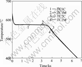
Fig.3 Measured and calculated temperature curves of TC1 and TC2
It can be seen from Fig.4 that the calculated temperature curve is identical with measured one at TC3, but there is a obvious deviation in the ascending segment at TC4. The maximum temperature difference between calculated temperature and measured one is 7.90 �� and most of temperature difference is less than 5.0 �� at TC3. The maximum temperature difference between calculated temperature and measured one is 8.80��, then 4.0-6.0 �� in the ascending segment and most are less than 3.0 �� at TC4. On one hand, this indicates that all of temperature differences are less than 9.0 �� (2��T) and satisfy the determination accuracy. On the other hand, the worse damping and lagging effect of the thermocouple in the sand mold induces the measurement error increasing. Consequently, the position of thermocouple should be closer to the interface of casting and sand mold so as to deduce the thermal resistance and decrease the measurement error by weakening the damping and lagging effect.
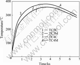
Fig.4 Measured and calculated temperature curves of TC3 and TC4
It can be seen from Fig.5 that the temperature curve of TC14 is identical with that of TC23, and the maximum temperature difference between TC14 and TC23 is only 1.0 ��. IHTC is a exponential function of temperature of casting surface, so it means IHTC at different position is basically equal at the same time.
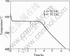
Fig.5 Calculated temperature curves of TC14 and TC23
Upon a comprehensive analysis, the Tikhonov regularization theory can efficiently solves the IHCP, decrease sensitivity to the input data, overcome the ill-posedness, and improve the accuracy and stability of the determination results. It is very important in the real engineering problem to simplify the determination process by setting up an appropriate IHTC mathematic model.
6 Conclusions
1) A new inverse method according to the Tikhonov regularization theory was presented. Moreover, a regularized functional was established and the regularization parameter was deduced. The functional was solved to determine the IHTC by using the sensitivity coefficient and Newton-Raphson iteration method.
2) The temperature measurement experiment was done, and the appropriate mathematical model of the IHTC was established. The determination results indicate that the Tikhonov regularization method is very efficient in overcoming the ill-posedness and ensuring the accuracy and stability of the solutions.
3) The direct calculations are very large with the number of variables increasing correspondingly during the inverse iteration. It is very important to decrease the number of direct calculations and improve the efficiency by employing an appropriate mathematic model of IHTC in the real engineering problem.
References
[1] BECK J V, BLACKWELL B, CLAIR C R S Jr. Inverse heat conduction-ill-posed problems [M]. New York: A Wiley-Interscience Publication, 1985.
[2] XIAO Ting-yan, YU Shen-gen, WANG Yan-fei. Numerical solution of inverse problem [M]. Beijing: Science Press, 2003. (in Chinese)
[3] LIU Ji-jun. The regularization method and application of ill-posedness problem [M]. Beijing: Science Press, 2005. (in Chinese)
[4] QUANPENG K E. Identification of interfacial heat transfer between molten metal and green sand by inverse heat conduction method [D]. Tuscaloosa: The University of Alabama, 2000.
[5] XUE Xing-jian. improvements on heat flux and heat conductance estimation with applications to metal castings [D]. Mississippi: Mississippi State University, 2003.
[6] BECK J V, BLACKWELL B, HAJI-SHEIKH A. Comparison of some inverse heat conduction methods using experimental data [J]. Int Comm Heat Mass Transfer, 1996, 39(17): 3649-3657.
[7] RAPPAZ M, DESBIOLLES J L, DREZET J M, GANDIN C A, JACOT A, THEVOZ P H. Application of inverse methods to the estimation of boundary conditions and properties [C]// Modeling of Casting, Welding and Advanced Solidification Processes�CVII. London: The Minerals, Metals and Materials Society, 1995: 449- 457.
[8] SHENEFELT J R, LUCK R, TAYLOR R P, BERRY J T, WOODBURY K A. Reducing uncertainty in the use of the inverse method of determining heat transfer coefficient data [C]// Modeling of Casting, Welding and Advanced Solidification Processes-IX. Aachen: United Engineering Foundation, 2000: 215-221.
[9] ADELEKE J, MUIKKU A. Inverse analysis for determination of interfacial heat transfer coefficient in complex three dimensional sand casting processes [C]// Modeling of Casting, Welding and Advanced Solidification Processes-X. Florida: The Minerals, Metals and Materials Society, 2003: 701-708.
[10] LIU Yuan, GUO Jing-jie, JIA Jun, LI Yan-Xiang, SU Yan-qing, DING Hong-sheng. Equivalent heat transfer coefficient at casting/Cu mould interface and temperature field simulation[J]. Trans Nonferrous Met Soc China, 2003, 13(5): 1119-1123.
[11] MAJCHRZAK E, MENDAKIEWICZ J, PIASECHA BELKHAYAT A. Algorithm of the mould thermal parameters identification in the system casting-mould-environment [J]. Journal of Materials Processing Technology, doi: 10.1016/j.jmatprotec.2005.02.021.
[12] SAHIN H M, KOCATEPE K, KAYIKCI R, AKAR N. Determination of unidirectional heat transfer coefficient during unsteady-state solidification at metal casting-chill interface [J]. Energy Conversion and Management, doi: 10.1016/j.enconman.2005.03.021.
[13] ZHOU Ji-ming, QI Le-hua, CHEN Guo-ding. New inverse method for identification of constitutive parameters [J]. Trans Nonferrous Met Soc China, 2006, 16(1): 148-152.
[14] WOODFIELD P L, MONDE M, MITSUTAKE Y. Implementation of an analytical two-dimensional inverse heat conduction technique to practical problems [J]. International Journal of Heat and Mass Transfer, doi: 10.1016/j.ijheatmasstransfer.2005.06.035.
[15] WIKSTROM P, BLASIAK W, BERNTSSON F. Estimation of the transient surface temperature and heat flux of a steel slab using an inverse method [J]. Applied Thermal Engineering, doi.10.1016/j.applthermaleng.2007.02.005.
[16] CHENG Wei, FU Chu-li, QIAN Zhi. A modified Tikhonov regularization method for a spherically symmetric three-dimensional inverse heat conduction problem [J]. Mathematics and Computers in Simulation, doi: 10.1016/j.matcom.2006.09.005.
[17] OKAMOTO K, LI B O. A regularization method for the inverse design of solidification processes with natural convection [J]. International Journal of Heat and Mass Transfer, doi: 10.1016/j.ijheatmasstransfer.2006.10.019.
[18] IJAZ U Z, KHAMBAMPATI A K, KIM M C, KIM S, KIM K Y. Estimation of time-dependent heat flux and measurement bias in two-dimensional inverse heat conduction problems [J]. International Journal of Heat and Mass Transfer, doi: 10.1016/j.ijheatmasstransfer. 2007.02.037.
Corresponding author: SUI Da-shan; Tel: +86-21-62813430-8029; E-mail: dasui@sjtu.edu.cn
