
J. Cent. South Univ. Technol. (2007)05-0685-05
DOI: 10.1007/s11771-007-0131-z ![]()
Adaptive learning with guaranteed stability for
discrete-time recurrent neural networks
DENG Hua(�� ��)1, WU Yi-hu(���廢)2, DUAN Ji-an(�μ���)1
(1. School of Mechanical and Electrical Engineering, Central South University, Changsha 410083, China;
2. School of Automobile and Mechanical Engineering, Changsha University of Science and Technology,
Changsha 410076, China)
Abstract��To avoid unstable learning, a stable adaptive learning algorithm was proposed for discrete-time recurrent neural networks. Unlike the dynamic gradient methods, such as the backpropagation through time and the real time recurrent learning, the weights of the recurrent neural networks were updated online in terms of Lyapunov stability theory in the proposed learning algorithm, so the learning stability was guaranteed. With the inversion of the activation function of the recurrent neural networks, the proposed learning algorithm can be easily implemented for solving varying nonlinear adaptive learning problems and fast convergence of the adaptive learning process can be achieved. Simulation experiments in pattern recognition show that only 5 iterations are needed for the storage of a 15��15 binary image pattern and only 9 iterations are needed for the perfect realization of an analog vector by an equilibrium state with the proposed learning algorithm.
Key words:
recurrent neural networks; adaptive learning; nonlinear discrete-time systems; pattern recognition ��
1 Introduction
Recurrent neural networks (RNNs) are among the most useful neural networks and have played important roles for discrete-time nonlinear processes in pattern recognition, modeling, adaptive control and adaptive filtering[1-8]. To train RNNs, two popular dynamic gradient methods, the backpropagation through time (BPTT)[9] and the real time recurrent learning (RTRL)[10], are frequently adopted. It is known that such on-line updating methods can be advantageous in problems that need only off-line training, e.g., for the standard backpropagation algorithm the on-line update is generally faster than the batch update[11]. However, if the weights of RNNs are adjusted on-line with such dynamic gradient methods, special consideration must be given to the stability of the adaptation because it is not ensured[12].
To ensure stable learning for RNNs, JIN and GUPTA[13] proposed a stable dynamic learning algorithm for discrete-time RNNs. The dynamic learning algorithm was based on the gradient descent method and named as dynamic back propagation (DBP) by NARENDRA and PARTHASARATHY[14]. By introducing explicit stability conditions into the weight updating algorithms, a checking phase was then added by JIN and GUPTA[13] to the learning process to guarantee the asymptotic stability of the equilibrium points during such a DBP learning procedure. However, long convergence time of such a stable DBP is often needed. In Ref.[7], a normalized RTRL algorithm that outperforms the standard RTRL algorithm was proposed. The stability of the normalized RTRL algorithm was proven by removing the second- and higher-order partial derivatives of the Taylor series expansion of the RNN output error and assuming that the weight updating error of a RNN was statistically independent of all variables with all on-line updated parameters[8]. Obviously, too many factors are neglected and the assumption is very strict.
In this paper, to solve varying nonlinear adaptive learning problems, a stable adaptive learning algorithm was proposed for discrete-time recurrent neural networks. Unlike the previous methods, the weights of the RNNs were updated online in terms of Lyapunov stability theory. The weight updating algorithm converged fast and was easily implemented. Two simulation examples in pattern recognition were also presented to validate the theoretical findings.
2 RNN and adaptive learning
2.1 RNN models
The discrete-time RNN model considered in this study has the following form:
![]() , i=1,2, ��, n (1)
, i=1,2, ��, n (1)
where
![]() ,
,
![]() ,
, ![]() ,
,
 ,
,
U0(k-1)= [u(k-1), ��, u(k-d0)]T,
U1(k-1)= [![]() , ��,
, ��, ![]() ]T,
]T,
Un(k-1)= [![]() , ��,
, ��, ![]() ]T,
]T,
0������1, 0��|��i|��+��,
![]() is the ith output and u(k) is an external input of the RNN, d denotes that the RNN has d inputs, ��i and ��i are undetermined constants, Wi and W0i are weights and thresholds and ��(?) is the activation function of the RNN with ��(u)=tanh (u). The neural network model (1) is a combination of the RNN model in Ref.[13] and the recurrent NARMA model in Ref.[8]. Model (1) is more general and thus can be used to solve a wide class of nonlinear discrete-time problems.
is the ith output and u(k) is an external input of the RNN, d denotes that the RNN has d inputs, ��i and ��i are undetermined constants, Wi and W0i are weights and thresholds and ��(?) is the activation function of the RNN with ��(u)=tanh (u). The neural network model (1) is a combination of the RNN model in Ref.[13] and the recurrent NARMA model in Ref.[8]. Model (1) is more general and thus can be used to solve a wide class of nonlinear discrete-time problems.
The following properties are associated with the RNN model (1), which will be used in the convergence proof of learning algorithms.
Property 1: ![]() in model (1) is bounded for all k.
in model (1) is bounded for all k.
Property 2: The region of the equilibrium points of model (1) is the n-dimensional hypercube[13] as follows:
![]() .
.
Property 3: -1��![]() ��1.
��1.
Property 1 can be verified by noticing that 0����i��1, 0��|��i|��+�� and -1����(vi(k))��1. This property shows that there are no unstable equilibrium states in model (1) if conditions 0����i��1 and 0��|��i|��+�� are satisfied. Property 2 shows the region of the equilibrium points and the approximation capability of the RNN. The approximation performance of the RNN cannot be guaranteed when the states of a nonlinear discrete-time process are outside the region. Therefore, parameters ��i and ��i must be properly chosen so that the region is large enough to include all the states of the nonlinear process. Property 3 will be used in the convergence proof of the proposed adaptive learning algorithm only. To prove property 3, re-write model (1) as
![]() .
.
Since -1����(vi(k))��1, the result is immediate.
2.3 Adaptive learning algorithm
Define the approximation error as
![]() (2)
(2)
where yi(k) is the ith target signal. The following learning algorithm is proposed to update the weights of the RNN model (1), which can guarantee the learning stability.
where i=1,2,��![]() , n,
, n, ![]() ,
,
![]() , 0����i��1 and 0�ܦ�i��1.
, 0����i��1 and 0�ܦ�i��1.
3 Stability and performance analysis
Stability and performance of the closed-loop system with RNN model (1) and weight updating law (3) are given in Theorem 1.
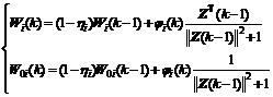
Theorem 1: For given RNN model (1) and input vector Z(k-1) of the RNN, if ![]()
![]() then adaptive learning algorithm (3) guarantees that ei(k)��0 as k����.
then adaptive learning algorithm (3) guarantees that ei(k)��0 as k����.
Proof First, it will be proven that the approximation error (2) approaches zero.
Choose a Lyapnuov candidate ![]() . The first difference of V(k) is given as
. The first difference of V(k) is given as
![]() (4)
(4)
Using model (1), one has
![]()
![]()
![]()
![]() (5)
(5)
Substituting the RNN adaptive learning law (3) into Eqn.(5), one obtains
![]()
![]()
![]()
![]() -
-
![]()
![]()
(6)
Using Eqn.(6), (4) becomes
![]() (7)
(7)
As 0�ܦ�i��1, from Lyapunov stability theory, Eqn.(7) shows that ![]() when
when ![]() .
.
Second, it will be proven that the RNN weights in the closed-loop system are bounded.
Re-write Eqn.(3) as follows:

(8)
Combining Eqn.(8) yields
![]() (9)
(9)
where
 ,
,
![]() .
.
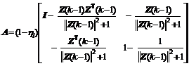
Choosing a non-singular matrix![]() , one obtains
, one obtains

As 0����i��1, all eigenvalues of matrix A1 are in the interval (-1, 1) and thus A is stable. On the other hand, in terms of Eqn.(6), ![]() in Eqn.(8) can be written as
in Eqn.(8) can be written as
![]()
![]()
![]() (10)
(10)
By property 3, -1��![]() ��1, then
��1, then ![]() exists. Therefore, 0��
exists. Therefore, 0��![]() ��+�� and the norm of B is bounded. As A is stable and B is bounded, the boundedness of Wi(k) and W0i(k) in Eqn.(9) is guaranteed, leading to the boundedness of Wi(k) and W0i(k) in Eqn.(3).
��+�� and the norm of B is bounded. As A is stable and B is bounded, the boundedness of Wi(k) and W0i(k) in Eqn.(9) is guaranteed, leading to the boundedness of Wi(k) and W0i(k) in Eqn.(3).
Remark 1: In RNN model (1), ��i is the time-constant or linear feedback gain of the ith neuron[13]. Usually, large time-constant result in that model (1) has slow dynamics. On the other hand, the capacity of the RNN model (1) decreases when ��i is too small. Therefore, typical value of the parameter ��i in adaptive learning algorithm (3) is between 0.1 and 0.4. After ��i is given, the parameter ��i is chosen to ensure that ![]() and thus theorem 1 holds.
and thus theorem 1 holds.
Remake 2: In adaptive learning algorithm (3), ��i is associated with the learning rate of RNN weights and ��i is associated with the convergence rate of the RNN output error. Generally, during adaptive learning, the oscillation of the weights becomes larger as ��i increases and the oscillation of the RNN output error becomes larger as ��i decreases. However, the learning stability is always guaranteed when 0����i��1 and 0����i��1. For most learning problems, the learning rate and the oscillation of the learning process must be considered together to ensure a fast and stable learning process. Simulation experiments show that typical values of the parameters ��i and ��i in adaptive learning algorithm (3) can be given between 0.1 and 0.5.
4��Simulation experiments
Example 1 (Binary image storage): A binary image pattern storage process[13] is studied here to illustrate the applicability of the proposed learning algorithm. As shown in Fig.1(a), a 15��15 binary image is used as the target pattern. The recurrent neural network is described by the following equation:
![]()
i, j=1, 2, ��, 15 (11)
where ![]() .
.
In RNN model (11), the double subscripts represent the two-dimension binary image. ![]() is a state of the neuron(i, j), which corresponds to the image unit (i, j).
is a state of the neuron(i, j), which corresponds to the image unit (i, j). ![]() is a weight between the neuron(i, j) and the neuron(h, l), and
is a weight between the neuron(i, j) and the neuron(h, l), and ![]() is a threshold of the neuron. In this example, the binary target pattern is desired to be stored directly at a stable equilibrium point of the network. For the initial stability of the network, all the iterative initial values of the weights and thresholds were chosen randomly in the interval [-0.001, 0.001] as in Ref.[13]. The parameters in Eqn.(11) and in the weight updating law (3) were chosen as
is a threshold of the neuron. In this example, the binary target pattern is desired to be stored directly at a stable equilibrium point of the network. For the initial stability of the network, all the iterative initial values of the weights and thresholds were chosen randomly in the interval [-0.001, 0.001] as in Ref.[13]. The parameters in Eqn.(11) and in the weight updating law (3) were chosen as ![]() ,
,![]() ,
,![]() ,
, ![]() . To observe the change of the binary image during the learning process, the pattern
. To observe the change of the binary image during the learning process, the pattern ![]() was employed to represent the binary image at the iterative instant k, where
was employed to represent the binary image at the iterative instant k, where ![]() if
if ![]() ��0.9, and yi,j=-1 if
��0.9, and yi,j=-1 if ![]() ��0.9.
��0.9.
Using the proposed adaptive learning algorithm, the dynamic learning process was completed at the iterative instant 5, and the 15��15 binary patterns were perfectly stored at a stable equilibrium point of the network. The proposed adaptive learning algorithm is very fast comparing with the learning algorithms in Ref.[13], in which 300 iterations are needed to complete the dynamic learning process. The recovered binary images at some iterative instant are depicted in Figs.1(b) and (c), and the error index and weight curves during the dynamic learning process are given in Fig.2. Both Figs.1 and 2 show that the proposed learning method has a very fast convergence speed and can be used effectively for large-scale pattern storage problems.
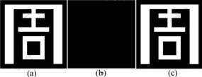
Fig.1 Target pattern and recovered binary images at different iterative instants
(a) Target pattern; (b) k = 2-4; (c) k = 5
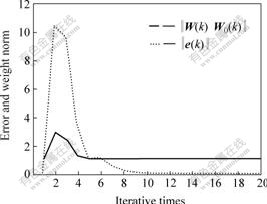
Fig.2 Error index and weight curves for example 1 during adaptive learning process
To check the stable equilibrium point of the network, the target pattern in Fig.1(a) is distorted by randomly and independently reversing each pixel of the pattern from +1 to -1 and vice versa with a probability of 0.1 as shown in Fig.3(a). Then the corrupted pattern is used as a probe for the trained RNN. After 4 iterations, the RNN converged onto the exactly correct form of the target pattern. The recollection of the corrupted target pattern is shown in Fig.3. Furthermore, it is found that, the larger the probability of reversing each pixel of the pattern is, the more the iterations are needed to converge onto the target pattern. For instance, 6 iterations are needed with a probability of 0.25 and 10 iterations with a probability of 0.40.
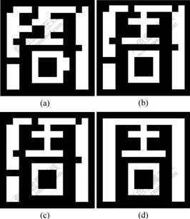
Fig.3 Recollection of corrupted target pattern
(a) Corrupted target pattern; (b) k=2; (c) k=3; (d) k=4
Example 2 (Analog vector storage): A two- dimensional analog vector storage problem[13] is considered in this example. The target pattern is t = [0.5, 0.8]T. A two-neuron model is employed, which is described as
![]() ������������ (12)
������������ (12)
where x1 and x2 are the states of the network. Two nonlinear equations are also introduced as follows, which are identical to that in Ref.[13].
![]() (13)
(13)
The objective of the simulation is to realize the target pattern t by a steady output vector y=[y1, y2]T, where ![]() and
and ![]() , and x=[x1, x2]T is an equilibrium state of the network. In Ref.[13], the initial values of the weights and thresholds were chosen randomly at the interval [-0.5, 0.5]. The parameters in Eqn.(12) and in the weight updating law (3) were chosen as ��i=0.2����i=1����i=0.25����i=0.1, i = 1, 2. Using the proposed adaptive learning method, the analog vector was perfectly realized by an equilibrium state with x1= 0.707 0 and x2 = 0.304 8, and the set of weights and thresholds were computed as
, and x=[x1, x2]T is an equilibrium state of the network. In Ref.[13], the initial values of the weights and thresholds were chosen randomly at the interval [-0.5, 0.5]. The parameters in Eqn.(12) and in the weight updating law (3) were chosen as ��i=0.2����i=1����i=0.25����i=0.1, i = 1, 2. Using the proposed adaptive learning method, the analog vector was perfectly realized by an equilibrium state with x1= 0.707 0 and x2 = 0.304 8, and the set of weights and thresholds were computed as
![]() ��
�� ![]() .
.
The error index and weight curves during the dynamic learning process are given in Fig.4, and the trajectory of the equilibrium points at different iterative instants is depicted in Fig.5. Fig.4 shows that only 9 iterations are needed to complete the dynamic learning process. However, using the methods in Ref.[13], the dynamic learning process was completed at a learning time k = 160 for the same storage problem. This example also illustrates that the proposed adaptive learning algorithm is stable and its convergence is fast.
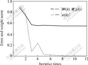
Fig.4 Error index and weight curves for example 2 during adaptive learning process
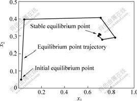
Fig. 5 Phase plane diagram of equilibrium point of network during adaptive learning (global stable equilibrium point is [0.7070, 0.3048])
5 Conclusions
1) The learning stability of the proposed adaptive learning algorithm can be guaranteed as the weight updating law of the RNNs is derived based on Lyapunov stability theory.
2) The proposed stable adaptive learning algorithm can be easily implemented with fast convergence for discrete-time recurrent neural networks.
3) Simulation experiments show that only 5 iterations are needed for the storage of a 15?15 binary image pattern and only 9 iterations are needed for the perfect realization of an analog vector by using the proposed learning algorithm. These results also validate the theoretical findings.
References
[1] GUPTA L, MCAVOY M. Investigating the prediction capabilities of the simple recurrent neural network on real temporal sequences[J]. Pattern Recognition, 2000, 33(12): 2075-2081.
[2] GUPTA L, MCAVOY M, PHEGLEY J. Classification of temporal sequences via prediction using the simple recurrent neural network[J]. Pattern Recognition, 2000, 33(10): 1759-1770.
[3] PARLOS A G, PARTHASARATHY S, ATIYA A F. Neuro-predictive process control using on-line controller adaptation [J] IEEE Trans on Control Systems Technology, 2001, 9(5): 741-755.
[4] ZHU Q M, GUO L. Stable adaptive neurocontrol for nonlinear discrete-time systems[J]. IEEE Trans on Neural Networks, 2004, 15(3): 653-662.
[5] LEUNG C S, CHAN L W. Dual extended Kalman filtering in recurrent neural networks[J]. Neural Networks, 2003, 16(2): 223�C239.
[6] LI Hong-ru, GU Shu-sheng. A fast parallel algorithm for a recurrent neural network[J]. Acta Automatica Sinica, 2004, 30(4): 516-522. (in Chinese)
[7] MANDIC D P, CHAMBERS J A. A normalised real time recurrent learning algorithm[J]. Signal Processing, 2000, 80(9): 1909-1916.
[8] MANDIC D P, CHAMBERS J A. Recurrent Neural Networks for Prediction: Learning Algorithms, Architectures and Stability[M]. Chichester: John Wiley & Sons, Ltd, 2001.
[9] WERBOS P J. Backpropagation through time: What it does and how to do it[J]. Proc IEEE, 1990, 78(10): 1550-1560.
[10] WILLIAMS R J, ZIPSER D. A learning algorithm for continually running fully recurrent neural networks[J]. Neural Computation, 1989, 1(2): 270-280.
[11] ATIYA A F, PARLOS A G. New results on recurrent network training: Unifying the algorithms and accelerating convergence[J]. IEEE Trans on Neural Networks, 2000, 11(3): 697-709.
[12] DENG Hua, LI Han-xiong. A novel neural network approximate inverse control for unknown nonlinear discrete dynamical systems[J] IEEE Trans on Systems, Man and Cybernetics��Part B, 2005, 35(1): 115-123.
[13] JIN L, GUPTA M M. Stable dynamic backpropagation learning in recurrent neural networks [J]. IEEE Trans on Neural Networks, 1999, 10(6): 1321-1334.
[14] NARENDRA K S, PARTHASARATHY K. Gradient methods for the optimization of dynamical systems containing neural networks[J]. IEEE Trans on Neural Networks, 1991, 2(2): 252-262.
Foundation item: Project(50276005) supported by the National Natural Science Foundation of China; Projects (2006CB705400, 2003CB716206) supported by National Basic Research Program of China
Received date: 2007-03-20; Accepted date: 2007-04-23
Corresponding author: DENG Hua, Professor, PhD; Tel: +86-731-8836499; E-mail: hdeng@csu.edu.cn
(Edited by ZHAO Jun)
