

J. Cent. South Univ. (2019) 26: 43-62
DOI: https://doi.org/10.1007/s11771-019-3981-2

Data driven particle size estimation of hematite grinding process using stochastic configuration network with robust technique
DAI Wei(��ΰ)1, 2, LI De-peng(�����)1, CHEN Qi-xin(������)1, CHAI Tian-you(������)2
1. School of Information and Control Engineering, China University of Mining and Technology,Xuzhou 221116, China;
2. State Key Laboratory of Synthetical Automation for Process Industries, Northeastern University,Shenyang 110819, China
 Central South University Press and Springer-Verlag GmbH Germany, part of Springer Nature 2019
Abstract:
As a production quality index of hematite grinding process, particle size (PS) is hard to be measured in real time. To achieve the PS estimation, this paper proposes a novel data driven model of PS using stochastic configuration network (SCN) with robust technique, namely, robust SCN (RSCN). Firstly, this paper proves the universal approximation property of RSCN with weighted least squares technique. Secondly, three robust algorithms are presented by employing M-estimation with Huber loss function, M-estimation with interquartile range (IQR) and nonparametric kernel density estimation (NKDE) function respectively to set the penalty weight. Comparison experiments are first carried out based on the UCI standard data sets to verify the effectiveness of these methods, and then the data-driven PS model based on the robust algorithms are established and verified. Experimental results show that the RSCN has an excellent performance for the PS estimation.
Key words:
Cite this article as:
DAI Wei, LI De-peng, CHEN Qi-xin, CHAI Tian-you. Data driven particle size estimation of hematite grinding process using stochastic configuration network with robust technique [J]. Journal of Central South University, 2019, 26(1): 43�C62.
DOI:https://dx.doi.org/https://doi.org/10.1007/s11771-019-3981-21 Introduction
Closed-loop optimization and control of particle size (PS) being key production quality indexes are hot topics in the mineral processing industry for years [1, 2]. Unfortunately, the real-time measurement of PS by online PS analyzer is often affected by the magnetic agglomeration characteristic of ore in hematite grinding process, thereby leading to unstable and inaccurate measurement. In fact, it is generally difficult, if not impossible, to achieve the closed-loop optimization and control in the absence of the reliable measurement [3, 4]. To tackle this problem, the relevant studies on PS estimation have been carried out. The conventional methods are based on first principle models [5, 6] with some ideal assumptions, which may result in a larger estimation error. As a consequence, it is well-received to employ data driven modeling techniques to solve the problem of PS estimation [7�C9].
The first generation of data driven PS model refers to linear regression model [10, 11]. But this model is usually hard to obtain a good estimation due to the nonlinear nature of hematite grinding process. In order to solve this nonlinear modeling problem of the hematite grinding process, the artificial neural network (ANN) [12�C14] and support vector machine (SVM) [7, 15] have been widely used to estimate the PS. Although a number of improved methods have evolved, there are still some problems, such as time-consuming training and inferior robustness. Therefore, it is essential to choose an appropriate data driven model for estimating the PS.
In the 90s of the last century, a special single-hidden layer feed-forward neural network (SLFN), named random vector functional link network (RVFLN), was proposed by PAO et al [16, 17]. The significant natures of RVFLN are as follows: 1) randomly assigning the hidden-node parameters (input weights and biases); 2) evaluating the output weights by solving a linear equation issue. A series of studies have shown that the RVFLN performs better in generalization and simple implementation than traditional SLFNs [18]. But, due to the fact that too small and too large networks will both attenuate the model quality, how to automatically choose an appropriate network architecture is crucial to application. To address this issue, there are three major approaches, i.e., pruning algorithms [19], constructive algorithms [20, 21] and regularization [22]. Actually, the constructive approach, which adds the hidden nodes one by one until a satisfactory solution is obtained, has a number of advantages over the others. Currently, the constructive algorithm has been introduced to the RVFLN thereby forming incremental RVFLN (IRVFLN). A new work reported in Ref. [23], however, has demonstrated the infeasibility of RVFLN and IRVFLN if the hidden-node parameters are selected randomly from a fixed scope. Thus, a novel network named stochastic configuration network (SCN) was proposed in Ref. [24]. Different with the IRVFLN, the SCN randomly selects hidden-node parameters with supervisory mechanism and adaptively assigns their scopes so that to ensure the selected hidden-node parameters proper. The universal approximation property of SCN has been proven in Ref. [24]. But, in almost all practical industrial systems, the presence of noises even the outliers is inevitable. Therefore, the robust problem of the current data driven modeling techniques should be solved sufficiently. That is to say, the further researches on how to improve the robustness of the SCN are of great essence.
Among the current researches, a robust version of SCN was developed in Ref. [25] by adopting weighted least squares method to evaluate the output weights. This paper contributes to prove that this robust SCN (RSCN) framework can successfully work in building a universal approximator. More precisely, the framework of the RSCN and its feature of universal approximation property have been presented first, and then three robust versions of SCN based M-estimation with Huber loss function, M-estimation with inter quartile range (IQR) and nonparametric kernel density estimation (NKDE) function respectively, are constructed. The data driven PS estimation model is built based on RSCNs method and validated by the actual grinding data that often contaminated by the outliers. Experimental results show that the data driven PS estimation model has high accuracy.
The remainder of this paper is organized as follows. In Section 2, a typical hematite grinding process studied is described and then its characterization analysis is achieved. The original IRVFLN and SCN are reviewed in Section 3. Section 4 details the framework and universal approximation property, which followed by three robust algorithms of RSCN. Section 5 reports the experimental results of RSCN on benchmark data sets and actual data of the hematite grinding process. Our concluding remarks are presented in Section 6.
2 Characteristic analysis of grinding process
The hematite grinding process studied in this paper operates in a closed loop. Figure 1 shows the flowsheet of this wet hematite grinding process: To begin with, fresh ore is fed continuously into a cylindrical mill together with a certain amount of mill water. Meanwhile, heavy metallic balls are loaded and tumbled in the mill to crush the coarse ore to finer sizes. After that, the mixed slurry is continuously discharged from the mill into the spiral classifier, where the slurry is separated into two streams namely overflow slurry and underflow slurry. The dilution water is used to adjust the classification concentration to maintain the overflow slurry with a proper proportion of finer particles. The underflow slurry with coarser particles is recycled back to the mill for regrinding. The overflow slurry is the product transported to the subsequent procedure.
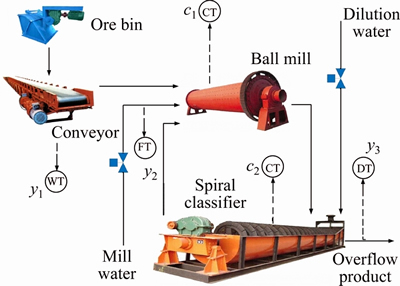
Figure 1 Flow chart of hematite grinding process (y1: fresh ore feed rate (t/h); y2: mill inlet water flow rate (m3/h); y3: classifier overflow concentration (%); c1: current through mill (A); c2: current through classifier (A); -T: instrument; F-, D-, C-, W-: flow rate, density, current and weighing, respectively)
In the above hematite grinding process, the PS (%) is easily affected by the operating parameters (namely, y1, y2 and y3), and ore properties (namely, size distribution B1 and grindability B2). Detailed analysis is as follows.
1) Influence of y1
The influence of y1 on PS can be seen from the grinding kinetic equation:
 (1)
(1)
where k and n are the parameters related to the probability of collision and ore properties, respectively; R0 and Rt represent the amount of non-grind and grinded coarse particles, respectively. It is easy to get that the larger Rt, the smaller PS. Therefore, Eq. (1) reveals that for the ores with constant grade R0, when k becomes smaller, PS will rise. In this condition, more particles are thus required to regrind, which accelerate flow velocity of slurry in the mill, thereby reducing the grinding time t. Consequently, PS will further decrease. In fact, y1 is usually expected to set as large as possible under the premise of qualified PS. However, increasing y1 alone will reduce k, thereby enhancing PS.
2) Influence of y2
y2 is a significant adjusting parameter for grinding concentration, which affects grinding viscosity to a strong extent. In fact, when the grinding viscosity changes, the flow rate of slurry will fluctuate, which could change the grinding time t. According to Eq. (1), therefore, PS will also change. Figure 2 showing the nonlinear relationship between the grinding concentration and the relative viscosity indicates the nonlinear mapping from y2 to PS.

Figure 2 Relationship between grinding concentration and relative viscosity
3) Influence of y3
According to the gravity beneficiation principle [26], the particles are graded by classifier based on the different settling rate of the particles with distinct sizes in the fluid. Actually, the settling rate directly affects the grading efficiency of the classifier. Because the slurry viscosity of classifier is a key factor for the settling rate, y3 that determines the slurry viscosity becomes a significant variable affecting PS. Figure 3 shows the nonlinear relationship between y3 and PS.
4) Influence of B1 and B2
Usually, PS is positively related to B1 under the same operating parameters. That is to say, the PS becomes larger with the increase of B1 and vice versa.

Figure 3 Relationship between y3 and PS
B2 describes the degree of ore variation under a certain grinding power consumption. Generally, the Bond work index [27] is often used to designate the B2, that is
 (2)
(2)
where W is the grinding power consumption and WI denotes the Bond work index; Q(��m) and F (��m) represent the sieve sizes that allow eighty percentage of the mineral particle passing in ore feed and grinding products, respectively. As we can see from Eq. (2), when Q and W remain unchanged, the fluctuation of WI depending on the B2 will cause the variation of F, that is, the change of PS.
Theoretically, a good estimated result can be achieved by using the above factors as model inputs. Unfortunately, B1 and B2 can not be measured in practice. Therefore, it is necessary to find other auxiliary variables that can approximately reflect the variation of B1 and B2 to estimate PS. Fortunately, the fluctuations of B1 and B2 can alter mill and classifier overload conditions, which should be recognized by mill current c1 and classifier current c2, respectively [28]. Therefore, the measurable c1 and c2 are utilized to replace B1 and B2 to realize the following nonlinear mapping.
 (3)
(3)
where f(��) is a unknown nonlinear function.
Magnetic agglomeration is a common characteristic of ferruginous ore. And hematite grinding process always suffers from corrupt measurements caused by the magnetic agglomeration characteristic, which leads to outliers. The motivation of this paper is to approximate the above mapping by using a SCN with robust technique.
3 Preliminaries
3.1 Review of IRVFLN
Let ��:={g1, g2, g3, ��} denote a set of real-valued functions and span(��) represent a function space spanned by ��. Let L2(D) represent the space of all Lebesgue measurable functions f={f1, f2, ��, fm}: Rd��Rm on a set  with the L2 norm defined as
 (4)
(4)
The inner product of f=[f1, f2, ��, fm]: Rd�� Rm and f is defined as
 (5)
(5)
For a given target function f: considering a given data set of training samples with inputs

 and the sampled output

 a SLFN with L-1 hidden nodes can be denoted as follows:
 (6)
(6)
where vj and bj are the parameters of the jth hidden node, which represent the input weights and the biases of hidden node, respectively; 
 is the output weight between the jth hidden node and the output nodes, gj is the activation function of the jth hidden node and fL�C1 denotes the output function when the (L�C1)th hidden unit is added.
According to Eq. (6), when the Lth hidden node is added, the output function of SLFN trained by IRVFLN is
 (7)
(7)
where
 (8)
(8)
and  represents the residual of the network
  and e0=y [23].
Remark 1: There is no doubt that the IRVFLN is indeed superior to the conventional RVFLN in terms of defining network structure. But the selection of random parameters of the hidden nodes should be specified and data dependent rather than assigning in a fixed scope [23]. Therefore, more attention should be paid for the assignment of the random parameters in RVFLN-based data driven modeling.
3.2 Review of SCN
Supposed that a SLFN with L�C1 hidden nodes has been built, i.e., ,and its current residual does not reach a satisfactory level, suffering from slow convergence rate. To tackle this issue, supervisory mechanism is employed by SCN, which provides an effective approach to select new hidden-node parameters (the input weights vL and biases bL) so that the learning modelwill obtain improved performance. The main work of SCN is presented in the following Theorem 1.
Theorem 1 ([24]). Supposed that span(��) is dense in L2 space and
 for some
  Given 0
 and
and  For L=1, 2, ��, denoted by
 q=1, 2, ��, m (9)
If the activation function gL is generated with the following constraints, namely, supervisory mechanism:
 (10)
(10)
and the output weights are calculated by
 (11)
(11)
Then, where
where

 And the optimal output weights ��* can be denoted as
 (12)
(12)
Remark 2: Different with the IRVFLN, the random parameters of SCN are selected under the supervisory mechanism to ensure that the randomized learning models have universal approximation property. Besides, as we can see from Eq. (10), the selection of the random parameters is constrained and data dependent. In other words, it is essential to adaptively select the scope of random parameters according to the different data sets. Even so, in the actual hematite grinding process, the collected data samples are usually contaminated by the outliers, which probably result in the unreliable estimation based on the SCN. Therefore, it is essential to improve the robustness of SCN.
4 RSCN based robust technique
It should be noted that outliers are gross errors which may give rise to the larger residuals for modeling. From Eq. (10) of Theorem 1, it can be seen that the inequality constraints are based on the residuals. The lager the residuals are, the looser the constraints are. Therefore, in the presence of outliers, the inequality constraints maybe too loose to effectively supervise the input weights and biases. In this condition, the conventional SCN constructed by Theorem 1 maybe no longer applicable for precisely modeling. A robust version of SCN was proposed in Ref. [25] by introducing a weighted form of residuals, its inequality constraints for the hidden-node parameters are presented in the following Theorem 2. This paper fully explores the universal approximation property of this version. Next, three different robust algorithms are adopted under this framework to obtain the penalty weight matrix, enabling RSCN to attenuate and even eliminate the negative influence of outliers on learner models.
4.1 Framework of RSCN
Based on the original SCN, the unified formula of RSCN can be mathematically expressed as the following Theorem 2 for a given N distinct multi-output samples.
Theorem 2. Supposed that span(��) is dense in L2 space and for some Given 0and For L=1, 2, ��, denoted by

 (13)
(13)
If the activation function gL is generated with the following constraints:
 (14)
(14)
and the output weights are calculated by

 (15)
(15)
Then, where fL=
 And
And represents the weighted form of
  when the number of hidden node is L�C1 for q=1, 2, ��, m. Of course, the ��* here has the same form with the Eq. (12). In addition,
  where P is the penalty weight matrix denoting the contribution of data samples to the model, and P can be denoted as
 (16)
(16)
Theorem 2 presents a robust framework for SCN. Besides the improved supervisory mechanism i.e., Eq. (14), this framework incorporates a weighted form of residual into the optimization model of output node parameters to enhance the robustness by using Eq. (15). The weighted form of residual ensures the reliability of samples for modeling by means of enlarging or decreasing the penalty weight. The following will give the solution of Eq. (15).

 (17)
(17)
where  denotes the hidden output and
Derivative of output weight  by Eq. (17), we can obtain

 (18)
(18)
Then, set Eq. (18) to zero, we can get that
 (19)
(19)
��* of multi-output RSCN can thus be written as


 (20)
(20)
Let 
 and then the according residuals
 . According to Ref. [24], we can get that the usage of Eq. (20) is more appropriate than Eq. (8) for calculating the output weight. Therefore, for the convenience of our proof about universal approximation property of RSCN, we can set some intermediate values
  and
and where
where  denotes the penalty weight of samples corresponding to the qth output node when the number of hidden node is L. Similar to the proof presented in Ref. [24], the proving process of Theorem 2 can be summarized as follows:
Proof. There is no doubt that 

 and as
  so we can get that
  is monotonically decreasing. Therefore, we have


 (21)
(21)
Therefore, can be further denoted as:
 (22)
(22)
Note that where
where  Based on Eq. (22), we can get that
  , that is,
This completes the proof.
Remark 3: First, this paper contributes to prove the universal approximation property of this RSCN framework. Second, under this framework, different versions of robust methods can be used. Three robust implementations are adopted herein, and the experiments hereinafter can verify that the framework of RSCN is better than IRVFLN and the original SCN, which proves the effectiveness of this robust framework. It is believed that not limited to the three weight functions, readers using other methods under this framework will also achieve good results. Comprehensive studies on the RSCN with respect to robust algorithms are described in the subsequent subsection.
4.2 Robust algorithms for SCN
This subsection details three RSCN algorithms, which are based on M-estimation using Huber loss function and M-estimation with IQR function, and NKDE function, respectively.
1) RSCN based on M-estimation with Huber loss function (Huber-RSCN)
The M-estimation [29, 30], using iterative weighted least squares as basic idea, was proposed by Huber first. Different from the conventional least squares giving same weight to each sample, the M-estimation adopts a new loss function to deal with the sample residuals. In the Huber-RSCN, the objective loss function is formulated as

 (23)
(23)
where Q(��) is the robust loss function of the residuals.  is the robust scale estimator and a widely used approach is to set
  where MAR denotes the median absolute residual and it can be obtained by
 (24)
(24)
where Med( ) is Median function.
The optimality condition of M-estimation can be presented as
 (25)
(25)
where ��(��) is the first-order derivation of Q(��), and represents the standardized residuals of ith sample corresponding to the qth output node.
In summary, the weight function can be defined as:
 (26)
(26)
Since the penalty weights are determined by the weight function in M-estimation, the selection of weight function directly affects the reliability of final output weights. The Huber loss function is adopted and presented as follows.
 (27)
(27)
where c is a positive adjustable parameter and is typically set as 1.345.
In this condition, the penalty weight function p(u) can be expressed as
 (28)
(28)
Worthy of note is that the initial penalty weight matrix P should be set to a matrix with all elements of 1. Combining Eq. (20), we can get that the output weight �� can be iteratively updated by using the following formula.


 (29)
(29)
where k represents the kth iterative alternation process.
2) RSCN based on M-estimation with IQR (IQR-RSCN)
For the IQR-RSCN, it has the similar implementation with the Huber-RSCN, but adopts a new weight function to calculate the sample weights. Compared with the Huber weight function that employs two residual size areas, the new weight function is a piecewise function with three residual size areas that are known as trusted area, suspect area and gross error area, respectively, and it can be presented as
 (30)
(30)
where c1 and c2 are two positive adjustable parameters and usually can be selected as c1=2.5 and c2=3.
In addition, ui,q can be acquired in the same way. But, different with the Huber-RSCN, the IQR-RSCN adopts the following formula to calculate 
 (31)
(31)
where the IQR denotes the difference between the 75th percentile and 25th percentile.
Although the Huber-RSCN and the IQR-RSCN present several differences, the same steps, which are presented in the Eq. (29), are adopted to calculate the output weight ��.
3) RSCN based on NKDE function (NKDE- RSCN)
Due to the fact that the distribution of sample residuals affected by the outliers is always far away from the overall residual distribution center, and it usually has a low density, so the probability density of the sample residuals can reflect reliability of sample data. To obtain the probability density of sample residuals, a NKDE function [31] can be adopted and the corresponding algorithm has been reported in [28]. This paper presents it to compare with the other algorithms.
In the initial phase, we need to set all the elements of matrix P as 1, and then calculate the standard residuals of the original model, that is

 (32)
(32)
Afterwards, the following probability density function of the residuals can be utilized.
 (33)
(33)
where  denotes the width of the estimated window,
 is the standard deviation of residuals, �� is Gaussian kernel function and presented as follows.
 (34)
(34)
For NKDE-RSCN, we still adopt an iterative alternation strategy between Eq. (29) and Eq. (33) to get sample reliability accurately. And the penalty weight matrix P can be calculated by Eq. (35).
 (35)
(35)
A brief summary for the weight functions of the above three algorithms are shown in the following Table 1. In essence, the weight functions taking the residual as an independent variable are employed to measure the contribution of training sample to modeling. That is, for framework of RSCN, when the (standardized) residual is smaller, the greater the contribution to the modeling is, the larger the corresponding weight function is, and vice versa.
Table 1 Specification of weight functions

Now we will have a summary on the above three different algorithms. In order to facilitate the algorithms description, the weighted form of residuals is replaced by using the The implementation steps of the three algorithms are summarized in the algorithm description.
Algorithm description
Given a regression data set of
 Set Lmax as the maximum number of hidden nodes, �� as the error tolerance, Smax as the maximum times of the random configuration of the hidden-node parameters, and Tmax as the maximum number of iterative alternation. Choose some positive values Z={lmin:��l:lmax}.
1
Given the initial weight matrix P which all the elements are set to 1, and calculating the initial residuals e. Let 0
2
While L��Lmax or ||e||>��, Do
3
For Do
Do
4
For i=1, 2, ��, Smax, Do
5
Randomly select the vL and bL from [�Cl, l]d and [�Cl, l], respectively.
6
Calculate the  (1), and set ��L=(1�Cr)/ (L+1).
7
If min{��L,1, ��L,2, ��, ��L,m}��0
8
Save vL and bL in W, and ��L in ��, respectively.
9
Else Go back to Step 5.
10
End If
11
End For
12
If W is not Empty
13
Find  and
and  maximizing ��L in ��, and construct
  .
.
14
Break (go to Step 18)
15
Else Randomly take ��=(0, 1�Cr) and let r=r+��, then return to Step 4.
16
End If
17
End For
Output Weight Determination
18
While j��Tmax or ||e||>��, Do
19
Huber-RSCN: Calculate the ��* by Eq. (29) and then obtain
20
Update the penalty weights by Eq. (28), renew P by Eq. (16) and let j=j+1 and e=
21
IQR-RSCN: Calculate the ��* by Eq. (29) and then obtain
22
Update the penalty weights by Eq. (30), renew P by Eq. (16) and let j=j+1 and e=
23
NKDE-RSCN: Calculate the ��* by Eq. (29) and then obtain .
.
24
Update the penalty weights by Eq. (35), renew P by Eq. (16) and let j=j+1 and e=.
25
End While
26
Let  .
.
27
End While
Note: (1) The variable q=1, 2, ��, m, let
 and
and  can be denoted as:
Based on Theorem 2, the hidden-node parameters can be stochastically configured by choosing a maximum ��L among multiple tests, subject to ��L,q��0, q=1, ��, m.
5 Performance evaluation
In this section, simulation experiments are carried out to confirm the robustness of RSCNs with respect to the outliers by comparing them with other two conventional algorithms, including IRVFLN and SCN. All experimental results are based on four benchmark data sets and an actual industrial grinding operation data set. The comparing experiments are conducted in MATLAB 2016a environment running on a PC that equips with a core i5, 3.4 GHz CPU, 8 GB RAM.
In the data preprocess, both the input and output data are normalized into [�C1, 1] before artificially adding different percentage of outliers. The maximum times of the random configuration of the hidden-node parameters Smax is set as 100; The error tolerance �� is set as 0.1; The parameter r is randomly generated between 0 and 1 using a random function. Settings of the other parameters will be given in the following specific experiments. For each algorithm, 50 independent trials are conducted and optimal values are obtained by using the method of cross validation.
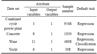
5.1 Benchmark test
Four real-world benchmark regression cases obtained from UCI Machine Learning Repository [32], including Combined cycle power plant, Concrete, Wine and Yacht, are used in the simulations. The detailed specifications of data sets are listed in Table 2. In the benchmark cases, the distributions of data are unknown and the greater part is not outlier-free. The training data and testing data of each case are randomly generated from its entire data set, separately. To further verify the robustness of model, training data sets need to be contaminated by means of artificially adding outliers. In this paper, the outlier percentage is successively selected from 0, 5%, 10%, 15%, 20%, 25% and 30% of the total number of training samples. It should be pointed out that the outliers can be generated by 
 where
where ��
�� index=1, ��, N, the index is randomly generated from the number of training samples N, and thus,
  is randomly selected from the output of normalized training samples;
 is also randomly generated and is added to the corresponding yindex. This means of data preprocess guarantees that the noise artificially added is more authentic, because ��index contains a positive and a negative distribution of values. Unlike training data sets, there is no need to add outliers to testing data sets.
Table 2 Specification of benchmark data sets
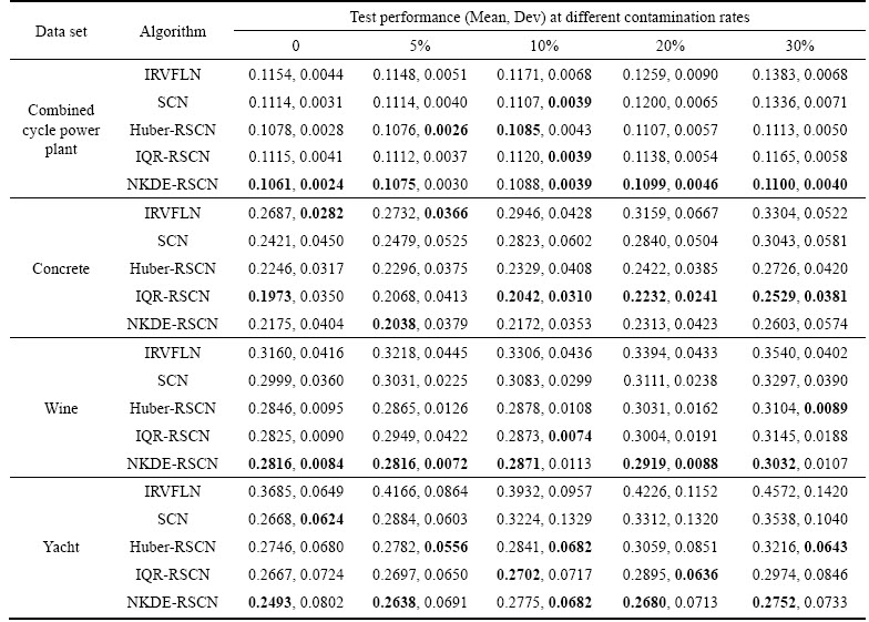
For each benchmark data set, Mean and Dev of the RMSE at each contamination rate are calculated to evaluate the performance of IRVFLN, SCN and the three robust algorithms. For each method and each data set, the experimental results are obtained with the optimal parameters (see in Table 3). In Table 3, Lmax is the maximum number of hidden nodes; is generated from some positive values; Tmax is the maximum number of iterative alternation.
Table 3 Partial optimization parameters

Mean and Dev of the RMSE are recorded in Table 4, and for each data set, the winner��s Mean and Dev are presented in boldface. Corresponding to Table 4, the simulation results are shown in Figures 4�C7. In detail, taking Figure 4 as an example, Figures 4(a)�C(e) are drawn based on boxplots of the algorithms under 50 independent trials. In Figure 4, as the level of outliers increasing, the testing RMSE shows an overall increasing tendency. The difference is that the testing RMSE of IRVFLN and SCN increase faster along with the growth of the outlier proportion, while the trends of three robust algorithms are relatively stable.
In order to evaluate which algorithm is best,the experiment results are further discussed based on Table 4. Considering the diverse impacts of outliers at low level contamination rate (0�C10%) and high level contamination rate (20%�C30%), the robustness of each algorithm is assessed via the following metrics: 1) Minimal Mean at each contamination rate; 2) Minimal Dev at each contamination rate; 3) Minimal range of Mean (maximum-minimum) at low level contamination rate; 4) Minimal range of Mean (maximum- minimum) at high level contamination rate.
Table 4 Comparison of mean values and standard deviations of RMSE
For each metric, lower is better. If an algorithm has a minimal value according to one metric then its score is assigned a winning score of 1, whereas other algorithms are assigned as 0. For instance, in the Concrete with contamination rate 10%, IQR-RSCN has a minimal Mean, then its score is set as 1, and all other algorithms are set as 0. For low and high level contamination rates, summations of all the scores of each algorithm are defined as subtotal (a) and subtotal (b), respectively. Each subtotal score expresses the outlier robustness of each algorithm at the corresponding level of contamination rate. The higher the score, the greater the robustness. The overall performance index is the summation of subtotals (a) and (b).
From Table 5, it can be seen that NKDE- RSCN has the highest total score among the comparative algorithms at all levels of contamination rates. IQR-RSCN comes second, followed by Huber-RSCN, and the original SCN and IRVFLN have low efficiency upon the outliers.
In order to compare the performance of different methods more intuitively, Figure 8 depicts the averaging testing RMSE under fifty independent trials. For each benchmark data set, the comparison results of different algorithms are plotted in the same simulation diagram, respectively. As observed from Figure 8, the averaging testing RMSE of IRVFLN and SCN ascends greatly along with the increase of the outlier percentage in most benchmark cases. In contrast, the variation of the outlier percentage has little effect on the accuracy of Huber-RSCN, IQR-RSCN and NKDE- RSCN. Moreover, comparing with IRVFLN and SCN, the three robust algorithms still have superior accuracy when the outlier percentage is at a higher level, although the averaging testing RMSE of all algorithms rise along with the increase of outlier percentage. It can also be easily found that among the three robust algorithms, in terms of robustness, NKDE-RSCN presents the best, IQR-RSCN exhibits better, Huber-RSCN is relatively inferior but still outperforms IRVFLN and SCN by a comprehensive comparison on the four benchmark data sets.

Figure 4 Testing RMSE comparison on benchmark data sets (Combined cycle power plant):
In summary, Huber-RSCN, IQR-RSCN, and NKDE-RSCN have strong robustness on different data sets, they thus can be used to establish the data-driven model for the PS estimation.
Remark 3: In theory, the SCN, Huber-RSCN, IQR-RSCN, and NKDE-RSCN should have a similar accuracy when the outlier percentage is 0,which is not consistent with the simulation results. This is because of the noises and outliers in raw data.
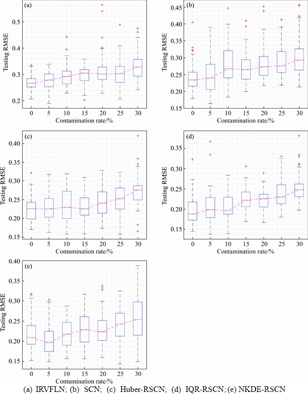
Figure 5 Testing RMSE comparison on benchmark data sets (Concrete):
5.2 PS estimation of hematite grinding process
In this section, the effectiveness of PS estimation using Huber-RSCN, IQR-RSCN and NKDE-RSCN will be displayed. In this application, the hematite grinding process data come from the hardware-in-the-loop simulation platform [33]. And the collected 800 samples are divided into 500 training samples and 300 testing samples. With the similar strategy of data preprocess, the normalized training data set randomly add outliers with different levels. In the light of readability, only the partial testing results are shown in Figure 9 and other trials of similar learning curves are same and omitted. Fifty independent trials are conducted and the relevant optimal parameters (see in Table 6) are acquired by the cross validation method. Mean and Dev of the RMSE are recorded in Table 7.

Figure 6 Testing RMSE comparison on benchmark data sets (Wine):
As we can see from Figure 9, it distinctly depicts the real values and estimated values of PS. The estimated values of three robust algorithms almost compactly surround the real values, while estimated values of the other two algorithms are away from the real values, especially IRVFLN. Besides, Figure 9 shows the robustness of Huber-RSCN, IQR-RSCN and NKDE-RSCN is excellent, followed by SCN that is still superior to IRVFLN. It is known from the above results, the three robust algorithms can achieve a satisfying accuracy, which demonstrates the potential application in the PS estimation of industrial grinding processes.
Furthermore, to demonstrate the universal approximation property of RSCN, the residual curves of three algorithms are shown at two certain levels of outliers in Figure 10. As observed from it, the tendencies of residual curves are substantially descending along with the growth of hidden nodes, which indicates that this robust version of SCNs provides a good convergence property. It should be pointed out that the three algorithms sharing the same framework adopt three different weight functions, respectively, which leads to the discrimination of residual curves. As described in Section 4.2, for Huber-RSCN and IQR-RSCN, their weight functions are piecewise functions, which is to make full use of useful information, limit the use of suspicious information and try to attenuate or eliminate harmful information. Unlike Huber-RSCN and IQR-RSCN, kernel density estimation is acquired by means of combining the probability density function of residuals with a Gaussian kernel function.

Figure 7 Testing RMSE comparison on benchmark data sets (Yacht):
Table 5 Comparison of score league of testing RMSE in benchmark cases
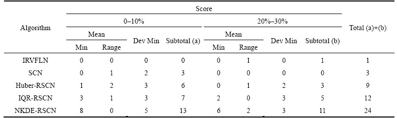
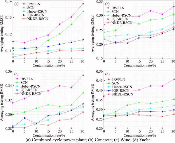
Figure 8 Averaging testing RMSE of all algorithms:
The residual curves of three algorithms is close to zero when the contamination rate is 0%; However, when the contamination rate is 15%, only IQR-RSCN makes the residual approach to zero. The conclusions from the perspective of weight function are as follows:
1) As for Huber-RSCN and IQR-RSCN, the weight function preferably contains three residual size areas: the trusted area whose weight remains unchanged, the suspect area whose weight is less than the initial weight and the gross error area whose weight should be approximately zero.
2) As for IQR-RSCN and NKDE-RSCN, their weight functions are based on completely different principles. As the contamination rate becomes higher, the residual curves of NKDE will be obviously worse, which results from the distribution of sample residuals affected by the high level of outlier and thus its density is no longer low.
That is to say, among the three algorithms, IQR-RSCN has the best performance for the hematite grinding process.

Figure 9 Testing results of five algorithms at 15% contamination rate:
Table 6 Partial optimization parameters

6 Conclusions
Data driven modeling techniques play a vital role in engineering applications, especially for complex industrial processes. As a particularly effective tool, neural network is widely applied to many fields. For the PS estimation, we concentrate on constructing stochastic configuration networks with robust techniques, including Huber-RSCN, IQR-RSCN and NKDE-RSCN, which adopt three different weight functions to improve their robustness, respectively. Based on different benchmark tests, the effectiveness of three robust algorithms is confirmed. The robust modeling techniques make the PS estimation a reality with satisfying accuracy. This means that the three robust algorithms can effectively tackle the problem of variable estimation in the hematite grinding processes. In addition, it is believed that those robust modeling techniques can also be applicable for other complex industrial processes.
Table 7 Comparison results of algorithms


Figure 10 Convergence performance:
References
[1] CHEN Xi-song, LI Qi, FEI Shu-min. Supervisory expert control for ball mill grinding circuits [J]. Expert Systems with Applications, 2008, 34(3): 1877�C1885.
[2] ZHOU Ping, DAI Wei, CHAI Tian-you. Multivariable disturbance observer based advanced feedback control design and its application to a grinding circuit [J]. IEEE Transactions on Control Systems Technology, 2014, 22(4): 1474�C1485.
[3] SHEN Ling, HE Jian-jun, YU Shou-yi, GUI Wei-hua. Temperature control for thermal treatment of aluminum alloy in a large-scale vertical quench furnace [J]. Journal of Central South University, 2016, 23(7): 1719�C1728.
[4] QIAO Jing-hui, CHAI Tian-you. Soft measurement model and its application in raw meal calcination process [J]. Journal of Process Control, 2012, 22(1): 344�C351.
[5] YUAN Zhi-tao, LI Li-xia, HAN Yue-xin, LIU Lei, LIU Ting. Fragmentation mechanism of low-grade hematite ore in a high pressure grinding roll [J]. Journal of Central South University, 2016, 23(11): 2838�C2844.
[6] WANG Xiao-li, GUI Wei-hua, YANG Chun-hua, WANG Ya-lin. Wet grindability of an industrial ore and its breakage parameters estimation using population balances [J]. International Journal of Mineral Processing, 2011, 98(1, 2): 113�C117.
[7] SUN Zhe, WANG Huan-gang, ZHANG Zeng-pu. Soft sensing of overflow particle size distributions in hydrocyclones using a combined method [J]. Tsinghua Science & Technology, 2008, 13(1): 47�C53.
[8] WANG Xin-hua, GUI Wei-hua, WANG Ya-lin, YANG Chun-hua. Prediction model of grinding particle size based on hybrid kernel function support vector machine [J]. Computer Engineering and Applications, 2010, 46(2): 207�C209. (in Chinese).
[9] ALDRICH C, MARAIS C, SHEAN B J, CILLIERS JJ. Online monitoring and control of froth flotation systems with machine vision: A review [J]. International Journal of Mineral Processing, 2010, 96(1): 1�C13.
[10] VILLAR R G D, THIBAULT J, VILLAR R D. Development of a softsensor for particle size monitoring [J]. Minerals Engineering, 1996, 9(1): 55�C72.
[11] WANG D, LIU J, SRINIVASAN R. Data-driven soft-sensor approach for quality prediction in a refining process [J]. IEEE Transactions on Industrial Informatics, 2010, 6(1): 11�C17.
[12] SBARBARO D, ASCENCIO P, ESPINOZA P, MUJICA F, CORTES G. Adaptive soft-sensors for on-line particle size estimation in wet grinding circuits [J]. Control Engineering Practice, 2008, 16(2): 171�C178.
[13] MARZBANRAD J, MASHADI B, AFKAR A, PAHLAVANI M. Dynamic rupture and crushing of an extruded tube using artificial neural network (ANN) approximation method [J]. Journal of Central South University, 2016, 23(4): 869�C879.
[14] KO Y D, SHANG H. Time delay neural network modeling for particle size in SAG mills [J]. Powder technology, 2011, 205(1): 250�C262.
[15] LIU Jin-peng, NIU Dong-xiao, ZHANG Hong-yun, WANG Guan-qing. Forecasting of wind velocity: an improved svm algorithm combined with simulated annealing [J]. Journal of Central South University, 2013, 20(2): 451�C456.
[16] PAO Y H, TAKEFUJI Y. Functional-link net computing: theory, system architecture, and functionalities [J]. Computer, 1992, 25(5): 76�C79.
[17] IGELNIK B, PAO Y H. Stochastic choice of basis functions in adaptive function approximation and the functional-link net [J]. IEEE Transactions on Neural Networks, 1995, 6(6): 1320�C1329.
[18] SCARDAPANE S, WANG Dian-hui. Randomness in neural networks: An overview [J]. Wiley Interdisciplinary Reviews: Data Mining & Knowledge Discovery, 2017, 7(2): 1�C18.
[19] REED R. Pruning algorithms��A survey [J]. IEEE transactions on Neural Networks, 1993, 4(5): 740�C747.
[20] KWOK T Y, YEUNG D Y. Objective functions for training new hidden units in constructive neural networks [J]. IEEE Transactions on Neural Networks, 1997, 8(5): 1131�C1148.
[21] KWOK T Y, YEUNG D Y. Constructive algorithms for structure learning in feedforward neural networks for regression problems [J]. IEEE Transactions on Neural Networks, 1996, 8(3): 630�C645.
[22] WEIGEND A S, RUMELHART D E, HUBERMAN B A. Generalization by weight-elimination with application to forecasting [C]// LIPPMANN R, MOODY J, TOURETZKY D S. Advances in Neural Information Processing Systems. San Mateo, CA: Morgan Kaufmann, 1991: 875�C882.
[23] LI Ming, WANG Dian-hui. Insights into randomized algorithms for neural networks: Practical issues and common pitfalls [J]. Information Sciences, 2017, 382�C383: 170�C178.
[24] WANG Dian-hui, LI Ming. Stochastic configuration networks: Fundamentals and algorithms [J]. IEEE Transactions on Cybernetics, 2017, 47(10): 3466�C3479.
[25] WANG Dian-hui, LI Ming. Robust stochastic configuration networks with kernel density estimation for uncertain data regression [J]. Information Sciences, 2017, 412�C413: 210�C222.
[26] PLITT L R. A mathematical model of the gravity classifier [C]// Proceedings of 17th International Mineral Processing Congress. Munich, 1991: 123�C135.
[27] BOND F C. Crushing and grinding calculations, Part I [J]. British Chemical Engineering, 1961, 6(6): 378�C385.
[28] DAI Wei, CHAI Tian-you, YANG S X. Data-driven optimization control for safety operation of hematite grinding process [J]. IEEE Transactions on Industrial Electronics, 2015, 62(5): 2930�C2941.
[29] ROUSSEEUW P J, CROUX C. The bias of k-step M-estimators [J]. Statistics & Probability Letters, 1994, 20(5): 411�C420.
[30] FAN Jun, YAN Ai-ling, XIU Nai-hua. Asymptotic properties for M-estimators in linear models with dependent random errors [J]. Journal of Statistical Planning & Inference, 2014, 148(148): 49�C66.
[31] SCOTT D W. Multivariate density estimation: Theory, practice, and visualization [M]. Houston, Texa: John Wiley and Sons, 2015.
[32] BLAKE C L, MERZ C J. UCI repository of machine learning databases, [DB/OL]. [1998]. http://www.ics.uci.edu/ ~mlearn/MLRepository.html.
[33] DAI Wei, ZHOU Ping, ZHAO Da-yong, LU Shao-wen, CHAI Tian-you. Hardware-in-the-loop simulation platform for supervisory control of mineral grinding process [J]. Powder Technology, 2016, 288: 422�C434.
(Edited by HE Yun-bin)
���ĵ���
����³�������������ij�����ĥ����������������ȹ���
ժҪ��������Ϊ������ĥ����̵Ĺؼ���������ָ�꣬���������ʵʱ�������⣬����������������磨Stochastic configuration network, SCN���Ļ����ϣ�֤����һ�ֻ��ڼ�Ȩ��С���˵�³��SCN(Robust SCN, RSCN)�����ܱƽ����ԣ����ֱ����Huber��ʧ������M���ơ��ķ�λ�ࣨInter quartile range, IQR����M���ƺͷDz������ܶȹ��ƣ�Nonparametric kernel density estimation, NKDE��������������ͷ�Ȩֵ���Ӷ��������RSCN�㷨����UCI�����ݼ��ϵ�ʵ���о������������㷨����Ч�ԡ�����RSCN�㷨���������������ij�����ĥ���������ģ�ͣ�ȡ�������õĹ���Ч����
�ؼ��ʣ�������ĥ����̣����ȣ������������(SCN)��³��������M���ƣ��Dz������ܶȹ���(NKDE)
Foundation item: Projects(61603393, 61741318) supported in part by the National Natural Science Foundation of China; Project(BK20160275) supported by the Natural Science Foundation of Jiangsu Province, China; Project(2015M581885) supported by the Postdoctoral Science Foundation of China; Project(PAL-N201706) supported by the Open Project Foundation of State Key Laboratory of Synthetical Automation for Process Industries of Northeastern University, China
Received date: 2017-12-08; Accepted date: 2018-04-26
Corresponding author: DAI Wei, PhD, Associate Professor; Tel: +86-13952235853; E-mail: daiwei_neu@126.com, weidai@cumt. edu.cn; ORCID: 0000-0003-3057-7225
Abstract: As a production quality index of hematite grinding process, particle size (PS) is hard to be measured in real time. To achieve the PS estimation, this paper proposes a novel data driven model of PS using stochastic configuration network (SCN) with robust technique, namely, robust SCN (RSCN). Firstly, this paper proves the universal approximation property of RSCN with weighted least squares technique. Secondly, three robust algorithms are presented by employing M-estimation with Huber loss function, M-estimation with interquartile range (IQR) and nonparametric kernel density estimation (NKDE) function respectively to set the penalty weight. Comparison experiments are first carried out based on the UCI standard data sets to verify the effectiveness of these methods, and then the data-driven PS model based on the robust algorithms are established and verified. Experimental results show that the RSCN has an excellent performance for the PS estimation.
