
���ڷǽṹ���������ά��ص������Ӧʸ������Ԫģ��
������1, 2��������1��������1, 3�����ɽ1
(1. ���ϴ�ѧ ��Ϣ��������ѧԺ������ ��ɳ��410083��
2. ��ɳ����ְҵ����ѧԺ �����ϵ������ ��ɳ��410014��
3. ��ʿ��������ѧԺ(EIH) ��������ϵ����ʿ ����ʿ��CH8092)
ժ Ҫ��
ժ Ҫ�������ܹ�ģ�⸴��ģ�͵ķǽṹ�������������ʸ����Ԫ����ά����Ӧ����Ԫ��ص��ģ���㷨��������ǣ����òв��͵ĺ���������ӳ�������������ϵĵ�Ԫ��ͨ�������������ĵ�Ԫ�������µ������µ������ظ���һ�����̣��Ӷ��õ����Ӿ�ȷ����ֵ������ظ���������ֱ���������ľ��ȴﵽԤ��Ҫ��Ϊֹ���Ӷ��������Ż�������Ԫ������COMMEMI 3D-1 MTģ�͵���ֵģ�⣬��֤�����㷨����ȷ�ԡ��о����������ͨ������Ӧ��������ܺ͵��������̣������㷨���Բ���������������ֵ��������������нϸߵľ��ȡ�
�ؼ��ʣ�
MT��ά�������ǽṹ��������ʸ������Ԫ���в��ͺ��������h-������Ӧ����Ԫ��
��ͼ����ţ�P631.322 ���ױ�־�룺A ���±�ţ�1672-7207(2010)05-1855-05
Three-dimension magnetotellurics modeling by adaptive edge finite-element using unstructured meshes
LIU Chang-sheng1, 2, TANG Jing-tian1, REN Zheng-yong1, 3, FENG De-shan1
(1. School of Info-physics and Geometrics Engineering, Central South University, Changsha 410083, China;
2. Department of Computer Science, Changsha Aeronautical Vocational and Technical College, Changsha 410014, China;
3. Institute of Geophysics, ETH-Swiss Federal Institute of Technology, Zurich CH8092, Switzerland)
Abstract: Based on unstructured grid which can simulate complex geoelectric models, the vector edge-based finite-elements were proposed. An adaptive finite element three-dimensional magnetotelluric modeling algorithm was introduced. The procedures are as follows: Element errors was estimated by a residual-based posteriori error on the coarse grid, and then elements with high error indicators were refined to generate a new grid. A new finite-element numerical processes were repeated on this new mesh to obtain more accurate and reliable numerical results. The iterative process was terminated until the accuracy of results on the final mesh became a required one. The COMMEMI 3D-1 model was tested to verify the correctness of the algorithm. The results show that for a complex three-dimensional electromagnetic model of the earth, using the adaptive mesh refinement and iterative solution procedure, the algorithm can generate iterative numerical results with high reliability.
Key words: magnetotelluric three-dimensional modeling; unstructured mesh; vector finite element method; residual based error estimation; h-adaptive finite element method
��Coggon[1]���������������е�����Ԫ�㷨(Finite element method, FEM)������FEM��ʼ�ڵ�ſ�̽����õ��㷺Ӧ��[2-5]��Badea��[6]���ýڵ��͵���������Ԫģ���˿ɿ�Դ��Ƶ��ص�ŷ���Mitsuhata��[7]���ڵ糡�����ƺʹų�ʸ���Ƶ�T-����ʽ���������Ե���������Ԫ��������ά��ص��ģ�ͣ�Nelson��[8-10]���÷ǽṹ����������������ʷֵļ�����ɢ��������⣬�Ӷ���������ά���ʸ������Ԫģ�⣻���Ң��[11]���ýڵ�������Ԫʵ������ά�ص��������ݵȣ����ǵ�[12]���û�����ߵ�ʸ������Ԫ������������ά��ص��ģ�͡�Ŀǰ�������������FEM�������1�����⣺��ֵ�������ľ�����ȫȡ���ڳ�ʼģ�͵���ɢ�������ڼĵ��ģ�ͣ����ھ�����Եõ����Ż�����ɢ�������ڸ���3D�ص�ģ�ͣ���ų�����̬�ͱ仯���Ƹ��ӣ���ƾ��Ϊ�������Եõ��Ż�����Ϊ����߸�������ĵ�ų����ȣ�������Խ��м���(h������Ӧ[13-14])������Ҳ�����ṩ�ֲ���ϵ�ų�����״����ʽ�����Ľ״�p(p������Ӧ[15-16])�������p������Ӧ���ԣ�h������Ӧ���Ը�����Ƕ�����еĴ���֮�У��Ӷ����̶�����ʱ�䡣Key��[17]����h������Ӧ�����˼��Զ�ά��ص��ģ�͵�ģ��������о���Li��[18]����һ�������뵽��ά�ɿ�Դ��ŷ�֮�С�������άģ�⣬�����������÷ǽṹ������������ں�������h������Ӧ���ܵ�3D��ص��ģ���㷨��
1 ��άMTʸ������Ԫ��ѧģ��
��ά MT ģ�͵�һ��ص�ṹ��ͼ1��ʾ�����У�![]() ��
��![]() ��
��![]() �ֱ�Ϊ�����㡢���µز�͵�����ص��쳣��ĵ絼�ʡ�
�ֱ�Ϊ�����㡢���µز�͵�����ص��쳣��ĵ絼�ʡ�
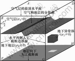
ͼ1 ��άMTģ�͵�һ��ص�ṹ
Fig.1 MT model of three-dimensional structure of general earth electricity
�ڿ�����͵��µز����糡���������ֿ��Ʒ���[19]��
![]() (1)
(1)
ʽ�У�EΪ�糡ǿ�ȣ�iΪ������![]() Ϊ��Ƶ�ʣ�
Ϊ��Ƶ�ʣ�![]() Ϊ���ɿռ�ŵ��ʣ�
Ϊ���ɿռ�ŵ��ʣ�![]() ΪMTģ�͵ĵ絼�ʡ�
ΪMTģ�͵ĵ絼�ʡ�
�������ۿɿ���ִ�м�Direlet�߽�����[20]��������ˮƽ�ز�ص�ṹ�ڱ߽��ϵĵ�ų�������Ϊ�߽�������
![]() (2)
(2)
ʽ�У�nΪ��߽���ⵥλ��������E0Ϊ��߽��ϸ�������֪�糡ǿ�ȡ�
����(1)��(2)������MT����ı�ֵ���⡣������ʸ�����ʽ![]() ��Gauss�ֲ����ֹ�ʽ�����Ӧ�ı�ֹ�ʽΪ��
��Gauss�ֲ����ֹ�ʽ�����Ӧ�ı�ֹ�ʽΪ��
![]() ��
��![]() (3)
(3)
ʽ�У�H(curl)ΪHilbert�ռ�������![]()
![]() ��
��![]() �������
Ϊ�������![]() Ϊƽ�����ӵ�Hilbert�ռ䣻bΪ˫���Ա���ʽ��fΪ�����Ա���ʽ��
Ϊƽ�����ӵ�Hilbert�ռ䣻bΪ˫���Ա���ʽ��fΪ�����Ա���ʽ��
�˴�����ʸ������Ԫ����ⷽ��(3)����ʾ�ĵ糡�ֲ���Ϊ�ˣ���Ҫ���������������ɢ��һϵ�������嵥Ԫ������ڵ�������Ԫ��֮ͬ�����ڣ������嵥Ԫ�е糡ǿ��E��ÿ���ߵ��������塣��������������嵥Ԫe�����Ѹõ�Ԫ�е糡�Ľ��Ʊ���ʽ��ʾΪ��
![]() (4)
(4)
ʽ�У�![]() ��
��![]() �ֱ��ʾ����ĵ糡�����Ͷ����ڵ�Ԫe�б�i�ϵ�ʸ����״������
�ֱ��ʾ����ĵ糡�����Ͷ����ڵ�Ԫe�б�i�ϵ�ʸ����״������
Ϊ�˱���α��ֵ�⣬�ڵ�������Ԫ������������ķ�������Ӵ��������Ѷȡ���ʸ������Ԫ��������ʸ����״����![]() ��ɢ��Ϊ0�������ܶȵ���ɢ��Ҫ����Ȼ�õ����㣻�����ǵ�ʸ����״����
��ɢ��Ϊ0�������ܶȵ���ɢ��Ҫ����Ȼ�õ����㣻�����ǵ�ʸ����״����![]() ������������ߵ�������������ˣ��糡�����������������õ����㣬�����������������������ʻ���ʸ����״�����������嵥Ԫ����Ч�ر������α�⡣
������������ߵ�������������ˣ��糡�����������������õ����㣬�����������������������ʻ���ʸ����״�����������嵥Ԫ����Ч�ر������α�⡣
MT ģ�����Ĵ������Է���Ϊ��
![]() (5)
(5)
���У�UΪ�����ڸ��������嵥Ԫ�ı��ϵ糡����δ֪������������A��B�ɸ�����Ԫ�Ĺ�������[21]��
![]() (6a)
(6a)
![]()
![]()
![]() (6b)
(6b)
ʽ�У�Bi������λ����Dirichlet�߽����ϵı߲�Ϊ0��
2 ���ڲв�ĺ���������
����N��d��lec���������Ե�Ԫ���������̿��Ա���Ϊ������TkΪ��������![]() ��һϵ�������������ʷֵ�Ԫ��FkΪ�����е�һϵ�������棻����Tk�ϵ�����Ԫ�ռ�UkΪ[21]��
��һϵ�������������ʷֵ�Ԫ��FkΪ�����е�һϵ�������棻����Tk�ϵ�����Ԫ�ռ�UkΪ[21]��
![]()
with ![]() (7)
(7)
��Tk�ϣ�����Ԫ����ɱ�ʾΪ�����Ek��Uk��ʹ������
![]() ,
, ![]() (8)
(8)
ʽ�У�![]() ��
��![]() ��
��
������ֵ������Ϊ��
![]() (9)
(9)
���Ƶ����ʺ���MTģ�͵ĺ���������Ϊ��
![]() (10)
(10)
ʽ�У�CΪһ����������ij�������T�ͦ�F�ֱ�Ϊ�����嵥Ԫ��������ľֲ���
3 ����Ӧ����
����h������Ӧ����Ԫ��MTģ�ͽ�����ֵģ�⣬�����ʷֲ���Լ����Delaunay������(DT)�ǽṹ����������Ӧ�ļ����㷨����������ģ�ͣ�ֻҪ������ʼ�����ȫ��������ֵ������h������Ӧ�������ԣ����������ȫ�Զ���⣬�����˹���Ԥ��
������������Tk�ϣ���������Ԫ�������Ek����������[22]�е�����������ۣ��ó���ǰ�����ϵ������ƣ����õ���Ԫ�ϵľֲ�������ָʾֵ��
![]()
![]()
![]() (11)
(11)
��Ӧ�أ�ȫ�����ָʾֵ�����������ָʾֵ�ֱ�Ϊ��
![]() (12)
(12)
![]() (13)
(13)
�����㵥Ԫ�������������������Ӧ�ļ��ܲ��ԣ������㷨������ͼ2��ʾ��
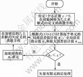
ͼ2 �����㷨����ͼ
Fig.2 Flow chart of calculation method
�㷨��Ӱ������Ӧ���ܹ��̵���ֹ����Ϊ1������С����![]() �ͼ����ܶ�����
�ͼ����ܶ�����![]() ��ͨ����˵��
��ͨ����˵��![]() С��1����
С��1����![]() �����ֵΪ0.5~0.7�����ڲ�ͬ�����⣬����
�����ֵΪ0.5~0.7�����ڲ�ͬ�����⣬����![]() Ҳ���ϴ�
Ҳ���ϴ�![]() ��[1��10-10, 0.1]�����⣬��ʵ�ʼ�������У�����������������n������ڴ�����M����������Ӧ��ֹ��һ��ȡn=10��M=500 MB��
��[1��10-10, 0.1]�����⣬��ʵ�ʼ�������У�����������������n������ڴ�����M����������Ӧ��ֹ��һ��ȡn=10��M=500 MB��
4 COMMEMI 3D-1 MTģ����ֵ ģ������
Ϊ�˼�ǿ�Աȷ�����ѡȡ����ͨ�õı�����ģ��COMMEMI 3D-1 model����ģ��[23]�����У��������쳣��ĵ�����Ϊ0.5 ?��m��Χ�ҵı���������Ϊ100 ?��m����Աȶȴ�1?200�����Ŀռ�ά�����£�x����Ϊ100 km��y����Ϊ100 km��z�����Ͽ�������Ϊ50 km����ز���Ϊ50 km��MT���߷ֲ���x��y�������ϣ����ȷ�Χ��Ϊ0~3 km��������Ϊ121������Ƶ��Ϊf=0.1 Hz��
����Ӧ���Ʋ���Ϊ��![]() =0.01��
=0.01��![]() =0.7��n=25��M=500 MB��ʵ�ʵ�������Ϊ20�����ڴ����Ϊ128.5 MB����ʼ����Ϊ10 553���ڵ㣬65 896����Ԫ�� 153 060���ߣ�����Ӧ���ܵĵ�12�������ģΪ13 238���ڵ㣬79 658����Ԫ��186 854���ߣ����һ��������Ϊ19 538���ڵ㣬113 281����Ԫ��267 798���ߡ�Ϊ�˼��㷽�㣬����ƽ̨ѡ��DELL D620�ʼDZ����Խ�����ֵģ�⣬����Ƶ��ֱ���32��16��8��4��2��1��
=0.7��n=25��M=500 MB��ʵ�ʵ�������Ϊ20�����ڴ����Ϊ128.5 MB����ʼ����Ϊ10 553���ڵ㣬65 896����Ԫ�� 153 060���ߣ�����Ӧ���ܵĵ�12�������ģΪ13 238���ڵ㣬79 658����Ԫ��186 854���ߣ����һ��������Ϊ19 538���ڵ㣬113 281����Ԫ��267 798���ߡ�Ϊ�˼��㷽�㣬����ƽ̨ѡ��DELL D620�ʼDZ����Խ�����ֵģ�⣬����Ƶ��ֱ���32��16��8��4��2��1��
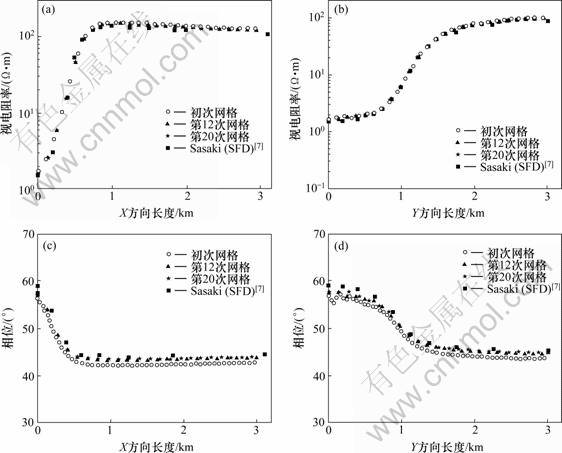
(a) x������ӵ�������; (b) y������ӵ�������; (c) x�������λ����; (d) y�������λ����
ͼ3 Ƶ��Ϊ0.1 Hz����������������MTģ�͵ĵر�����ϵ���λ���ӵ���������
Fig.3 Phase and resistivity curves containing uneven surface cube measuring point when frequency is 0.1 Hz
0.5��0.25��0.1 Hz���ܺ�ʱΪ317.461 4 s�����У����������Dz���tetgen���������ʷ֣��Զ����ܲ�ȡ���ּ��ܣ�ʱ�������1 s���Զ�Ƶ���������ʱ56.811 0 s����С��ʱ23.319 5 s��ƽ����ʱ35.273 5 s��
ͨ��ģ��õ�3D-1ģ�͵�����Ӧ��������ĺ������ֲ�����0.1 HzƵ��ģ��������з������ڳ�ʼ�����ϵĵ�Ԫ���ϴ�ƽ�����Ϊ74.48%��������Ϊ165.00%����ˣ��ϴ�����ֲ���ʹ��Ƶ�����Ӧ���ܲ�������������������ĵ�Ԫ����һ����ڵ�12��20�������Ͽ������Կ������ڵ�12�������ϣ���Ԫƽ��������3.33%�����������6.12%���ڵ�20�������ϣ���Ԫƽ��������0.93%,���������3.98%����ƽ�����С�ڸ����1%����ˣ����ܹ�����ֹ����ֵģ������Sasaki��Ա�ģ�����ü��������Ǻ�(��ͼ3�е�Sasaki(SFD))[7]��
ע����߸����ĵ�Ԫ��û����������Ӧ���ܹ��̵����ж��������������ܡ���һ�����²��߸�����ֵ�������(��ͼ3)���ӵ����ʵ�ƽ�����ӳ�ʼ�����ϵ�3.49%����Ϊ��12�������ϵ�0.87%�����ǣ�����������ټ��ܣ��ӵ�����ƽ�����ʼ�ձ�����0.50%~1.00%����λ���ߵ�ƽ�����ӳ�ʼ�����ϵ�1.23%����Ϊ��20��ʱ��0.21%�����ǣ�����������ټ��ܣ���λ����ƽ�����ʼ�ձ�����0.20%~0.50%��
5 ����
(1) ���ݵ糡�ֿ��Ʒ��̺ͱ߽����������û���ʸ����״�����������嵥Ԫ����ʸ����״������ɢ��Ϊ0�������ܶȵ���ɢ��Ҫ��ͱ���Ȼ���㣬��ˣ�����Ч�ر���α��ij��֣��Ӷ���������άMTʸ������Ԫ��ѧģ�͡�
(2) �Ƶ������ڲв����ά��ص��ʸ������Ԫ���������ƹ�ʽ��Ϊ��ά��ص������Ӧʸ������Ԫ��ֵģ���ʵ�ֵ춨�˻�����
(3) ����ȫ�ǽṹ�������嵥Ԫ�ʷּ��Ż������ϣ������ά��ص��ʸ������Ԫ���������ƹ�ʽ������˻��ڷǽṹ���������ά��ص��h������Ӧʸ������Ԫ������ԣ���֤�˶Ը��Ӵ�ص��ģ����ֵ����ľ��ȺͿɿ��ԡ�
(4) ���ģ�͵ĸ����������ϲ�Ӱ�췽���������ԣ��ҿ��ԴﵽԤ�ڵļ��㾫�ȡ��ɼ���h������Ӧʸ������Ԫ���Ա�֤����ģ�͵ļ��㾫�Ⱥ��ٶȣ����й�����Ӧ��ǰ����
�ο����ף�
[1] Coggon J H. Electromagnetic and electrical modeling by the finite element method[J]. Geophysics, 1971, 36(1): 132-145.
[2] Pridmore D F, Hohmanns G W, Ward S H, et al. An investigation of finite-element modeling of electric and electromagnetic data in three dimensions[J]. Geophysics, 1981, 46(7): 1009-1024.
[3] ���DZ. ����Ԫ�ط��ڵ編�⾮�е�Ӧ��[M]. ����: ʯ��ҵ������, 1980: 15-67.
LI Da-qian. The application of finite element method in electric well logging[M]. Beijing: Petroleum Industry Press, 1980: 15-67.
[4] ������, �Ź���. ���Ӽ�����ڵ編��̽�е�Ӧ��[M]. �人: �人����ѧԺ������, 1987: 51-99.
LUO Yan-zhong, ZHANG Gui-qing. Application of electronic computer in electrical prospecting[M]. Wuhan: Press of Wuhan College of Geology, 1987: 51-99.
[5] ������. ���������е�����Ԫ��[M]. ����: ��ѧ������, 1994: 23-28.
XU Shi-zhe. Finite element method in geophysics[M]. Beijing: Science Press, 1994: 23-28.
[6] Badea E A, Everett M E, Newman G A, et al. Finite-element analysis of controlled-source electromagnetic induction using Coulomb-gauged potentials[J]. Geophysics, 2001, 66(3): 786-799.
[7] Mitsuhata Y, Uchida T. 3D magnetotelluric modeling using the T-�� finite-element method[J]. Geophysics, 2004, 69(1): 108-119.
[8] Nelson E M. Advances in 3D Electromagnetic finite element modeling[C]//Proceedings of the IEEE 1997 Particle Accelerator Conference. Vancouver, Canada, 1998: 1837-1840.
[9] Sugeng F. Modeling the 3D TDEM response using the 3D full-domain finite-element method based on the hexahedral edge-element technique[J]. Exploration Geophysics, 1998, 29(4): 615-619.
[10] Yoshimura R, Oshiman N. Edge-based finite element approach to the simulation of geoelectromagnetic induction in a 3-D sphere[J]. Geophysical Research Letters, 2002, 29(3): 1039-1045.
[11] ���Ң, �ܱ�, ������. ��ά�ص��������ʲ�������Ԫ��ֵģ��[J]. �����ѧ, 2001, 26(1): 73-77.
RUAN Bai-yao, XIONG Bin, XU Shi-zhe. Finite element method of modeling resistivity sounding on 3D geoelectic section[J]. Earth Science, 2001, 26(1): 73-77.
[12] ����. ����ʸ������Ԫ�ĸ�Ƶ��ص�ŷ���ά��ֵģ��[D]. ��ɳ: ���ϴ�ѧ��Ϣ��������ѧԺ, 2008: 35-62.
WANG Ye. A study of 3D high frequency magnetotellurics modeling by edge-based finite element method[D]. Changsha: Central South University. School of Info-physics and Geometrics Engineering, 2008: 35-62.
[13] Zienkiewicz O C, Zhu J Z. Adaptive and mesh generation[J]. Int J Num Meth Eng, 1991, 32(4): 783-810.
[14] Tani K, Yamada T. H-version adaptive finite element method using edge element for 3D non-linear magnetostatic problems[J]. IEEE Transactions on Magnetics, 1997, 33(2): 1756-1759.
[15] Szabo B A. Mesh design for the p-version of the finite element method[J]. Computer Methods in Applied Mechanics and Engineering, 1986, 55(1): 181-197.
[16] WEN Dai-gang, JIANG Ke-xun. P-version adaptive computation of FEM[J]. IEEE Transactions on Magnetics, 1994, 30(5): 3515-3518.
[17] Key K, Weiss C. Adaptive finite-element modeling using unstructured grids: The 2D magnetotelluric example[J]. Geophysics, 2006, 71(6): 291-299.
[18] LI Y G, Key K, Constable S. An adaptive finite element modeling of 2-D marine controlled-source electromagnetic fields[C]//18th IAGAWG 1.2 Workshop on Electromagnetic Induction in the Earth. El Vendrell, Spain, 2006: S3-S14.
[19] Harrington R F. Time harmonic electromagnetic fields[R]. New York: McGraw-Hill Book Co, 1961: 37-85.
[20] Nam M J, Kim H J, Song Y, et al. 3D magnetotelluric modeling including surface topography[J]. Geophysical Prospecting, 2007, 55(2): 277-287.
[21] LIU Chang-sheng, REN Zheng-yong, TANG Jing-tian, et al. Three-dimensional magnetotellurics modeling using edge-based finite element unstructured meshes[J]. Applied Geophysics, 2008, 5(3): 170-180.
[22] CHEN Zhi-ming, WANG Long, ZHENG Wei-ying. An adaptive multilevel method for time-harmonic Maxwell equations with singualarities[J]. Siam J Sci Comput, 2007, 29(1): 118-138.
[23] Zhdanov M S, Varentsov I M, Weaver J T, et al. Methods for modeling electromagnetic fields Results from COMMEMI��the international project on the comparison of modeling methods for electromagnetic induction[J]. Journal of Applied Geophysics, 1997, 37(3/4): 265-271.
�ո����ڣ�2010-03-31�������ڣ�2010-06-10
������Ŀ�����Ҹ����о���չ�ƻ�(��863���ƻ�)��Ŀ(2006AA06Z105��2007AA06Z134)��������Ȼ��ѧ����������Ŀ(40804027)������ʡ�Ƽ��ƻ���Ŀ(2008FJ4181)������ʡ�ߵ�ѧУ��ѧ�о���Ŀ(08D008)������ʡ��Ȼ��ѧ�����ص�������Ŀ(09JJ3084)
ͨ�����ߣ����ɽ(1978-)���У����������ˣ���ʿ�������ڣ����µ�ŷ���̽�о����绰��0731-88836145��E-mail: fengdeshan@126.com
