
J. Cent. South Univ. (2016) 23: 1990-2000
DOI: 10.1007/s11771-016-3256-0

A variation pixels identification method based on kernel spatial attraction model and local entropy for robust endmember extraction
ZHAO Chun-hui(�Դ���), TIAN Ming-hua(������), QI Bin(���), WANG Yu-lei(������)
College of Information and Communication, Harbin Engineering University, Harbin 150001, China
 Central South University Press and Springer-Verlag Berlin Heidelberg 2016
Abstract:
A variation pixels identification method was proposed aiming at depressing the effect of variation pixels, which dilates the theoretical hyperspectral data simplex and misguides volume evaluation of the simplex. With integration of both spatial and spectral information, this method quantitatively defines a variation index for every pixel. The variation index is proportional to pixels local entropy but inversely proportional to pixels kernel spatial attraction. The number of pixels removed was modulated by an artificial threshold factor ��. Two real hyperspectral data sets were employed to examine the endmember extraction results. The reconstruction errors of preprocessing data as opposed to the result of original data were compared. The experimental results show that the number of distinct endmembers extracted has increased and the reconstruction error is greatly reduced. 100% is an optional value for the threshold factor �� when dealing with no prior knowledge hyperspectral data.
Key words:
variation pixels; hyperspectral; simplex; variation index; local entropy; kernel spatial attraction��
1 Introduction
Airborne and satellite hyperspectral sensors collect significant quality data of observed land scene [1] with precision diagnostic power of spectral resolution (0.4 to 2.5 ��m) but coarse spatial resolution (e.g. 5 to 20 m). For an observed land scene, the distinct substances (e.g. grass, sand, oil, water and corn), treated as representative substances, are termed endmembers. Due to the coarse spatial resolution, a mass of pixels contain more than one material. Thus, extracting pure spectral pixel and estimating abundance fractions for mixing pixel are critical for hyperspectral interpretation.
Endmember extraction techniques aim at searching out high purity spectral signatures from hyperspectral imagery. A large number of methods have been developed to extract endmembers with [2-6] or without [7-9] assumption of the presence of endmembers. Current endmember extraction technologies suffer two issues: 1) large amounts of data enlarge the searching space and furtherly reduce the efficiency [10-11] and 2) due to the difference results from illumination conditions, environmental factors, atmospheric conditions, variations in topography and moisture content of crops, spectrum signatures show variability [12] which puts back accuracy of endmember extraction. Pixels with high variability and interference data interpretation are called variation pixels.
Geometrically, the hyperspectral data cube is of a convex simplex with endmembers located at the vertexes [13]. In recent years, many approaches have been proposed for endmember extraction. N-FINDR algorithm calculates simplex volume iteratively [6]. Pixels which construct the maximum simplex volume are extracted as endmembers. This algorithm is constraintted by both the initial endmember set and the endmember sequence. PPI algorithm projects the hyperspectral data cube into thousands of random vectors [2]. The probability of one pixel being extracted as an endmember is proportional to the times of extreme projection documented. In contrast, OSP algorithm projects the hyperspectral data cube into an orthogonal subspace, then the pixel with the maximum projection value is extracted as an endmember [4]. The VCA algorithm takes illumination variability into account by introducing a scale factor [5]. Substantially, it is a geometrical projection method. Besides, tremendous approaches have been developed, such as simplex growing algorithm (SGA) [14], automatic morphology endmember extraction (AMEE)[15], maximum volume by householder transformation (MVHT) [16], genetic orthogonal projection (GOP) [17], random N-FINDR (RN-FINDR) [18] and modified vertex component analysis (MVCA) [19]. However, current endmember extraction methods can hardly account for the variability of pixels.
The pixels variability, defined as two types: 1) intra- class variability and 2) inter-class variability [20], is resulted from a variety of reasons. Variable illumination condition is a major source of pixels variability originated by topography and surface roughness of objects [21]. Besides, crop conditions, water content, the canopy structure, leaves distributions, atmospheric and some temporal factors can result in pixels variability [12].
To depress pixels variability, ROBERTS et al [22] used multiple endmember spectral mixture analysis (MESMA) on mapping. This method allows a variable type and a variable number of endmembers for per pixel unmixng. Similarly, ASNER et al [23] selected endmembers randomly from spectral library and operated unmixng procedure several times, termed automated Monte Carlo unmixing (AutoMCU). BATESON et al [24] proposed endmember bundles for unmixing from a perspective that traditional single endmember is represented by one endmember bundle. However, the challenge of this method is that a mass of different endmember combinations are required to be tested. Besides, some scholars presented solutions from a view of optimal band set and transformation. JIN et al [25] exploited a Fisher discriminant approach (FDA). The FDA measures the scatter degree within endmembers. Researchers also conducted methods including support vector machines (SVMs) [26] and sparse theory [27].
However, there is lack of detailed references about variation pixels identification. This work proposes a variation pixels identification method based on the kernel spatial attraction and local entropy. Different from current existing data preprocessing techniques [28-31], the proposed method focuses on variation pixels identification and removing instead of data compaction.
2 Methodology
Variation pixels mislead the volume evaluation of a simplex. As shown in Fig. 1(a), point A, point B and point C are the true endmembers related to three distinct substances. The solid triangle S is the true simplex. The dotted triangle S�� is an error simplex extracted when the variation pixel A��is extracted as an endmember. Variation pixel A�� and point A essentially belong to the same category but extracted as two distinct endmembers. In spectral space, the existence of variation pixels results in an irregular simplex (Fig. 1(a)). Commonly, the volume of an error simplex is larger than the true simplex. Figure 1(b) shows that in spatial space, variation pixels easily exist on the boundary of different substances [31]. Pure pixels with low variability locate in the homogeneous areas (the grid squares) while variation pixels exhibit instability, away from homogeneous areas. The homogeneous areas are defined as regions in which all the pixels�� spectral dissimilarities are below a given threshold [31]. Specifically, endmembers with a high probability exist in the homogeneous areas.
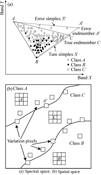
Fig. 1 Distributions of variation pixels:
2.1 Kernel spatial attraction model used in fuzzy probability space
Spatial attraction model is introduced in detail and used for sub-pixel mapping [32]. A larger spatial attraction indicates a higher similarity of the current center pixel with its neighbor pixels. To further access the spatial homogeneity, the kernel spatial attraction model is proposed.
Firstly, the hyperspectral data cube X, in M��N��L size, where M is the number of rows, N is the number of columns of hyperspectral imagery in spatial space and L denotes the total number of bands, is transformed into fuzzy probability space using fuzzy k-mean clustering [33] method.
The cost function J(Q, C) is
 (1)
(1)
where  (i=1, ��, M, j=1, ��, N, v=1, ��, D) is the fuzzy probability matrix; D is the number of classes;
 is the fuzzy probability of pixel ri,j corresponding to class v; is subjected by
 and
and 
 is an exponent parameter. In this work ��=2. Matrix C is the clustering center matrix C=[cv] (v=1, ��, D), where cv is the clustering center vector of class v. The number of classes D for a hyperspectral data cube can be calculated by virtual dimensionality (VD) analysis [34].
  is defined as Euclidean distance between pixel ri,j and the clustering center vector cv and it can be computed by
 (2)
(2)
After fuzzy k-mean clustering, each pixel vector ri,j gains a fuzzy probability vector Ri,j, which describes the similarity of ri,j with the clustering center matrix C as
 (3)
(3)
Hence, the original data cube X can be represented by fuzzy probability matrix
 (Fig. 2). Ql is the fuzzy probability matrix corresponding to class l. In X, ri,j is a L��1 column vector with elements of bands reflectance. In the fuzzy probability space Q, Ri,j is a D��1 column vector with elements of fuzzy probabilities.
Then, a sliding calculation window in m��m size is adopted (m=3). There are m2 pixels totally in the current calculation window (Fig. 2). In Fig. 2, Ri,j is fuzzy probability vector and Ra,b is the neighbor fuzzy probability vector (a=i-(m-1)/2, ��, i+(m-1)/2; b=i-(m-1)/2, ��, i+(m-1)/2 and a��i, b��j);  is the spatial distance between Ri,j and Ra,b. The attraction h(ij),(ab) between Ri,j and Ra,b is


 (4)
(4)
Scalar  denotes the weight coefficient. Vv(ri,j) is the fuzzy probability character of pixel ri,j related to class v.
Furthermore, to improve the nonlinearity, the Gaussian radial basis function (GRBF) is imported into formula (4). The GRBF is
 (5)
(5)
Then, the whole kernel spatial attraction Hij for the center pixel ri,j is an average of all the respective attraction h(ij),(ab). The weight coefficient is defined as the reciprocal of the Euclid distance and t equals 2. Thus,


 (6)
(6)
With the calculation window sliding through the whole imagery, each pixel ri,j gains a kernel spatial attraction value Hi,j, which reflects the spatial homogeneity character. A smaller Hi,j indicates ri,j located in a lower spatial homogeneity area with higher variability.

Fig. 2 Kernel spatial attractions model
2.2 Local entropy definition for hyperspectral imagery
The Shannon��s entropy theory measures the amount of uncertainty of a random vector through the probability distribution. Local entropy reflects the information content of the current center pixel with its spatial neighbors. An advanced local entropy concept for hyperspectral imagery is proposed in this section.
For the current center pixel ri,j located at the i-th row and j-th column within local area G (m��m size), the local entropy EG(ri,j) is
 (7)
(7)
Particularly,
 ,
,
 (t=0, 1, 2, ��, m) (8)
where  is the entropy of ri,j related to band k;
  is the reflectance value of ri,j in band k;
  denotes the reflectance probability of pixel ri,j. A higherlocal entropy indicates a higher variability.
2.3 Variation pixels identification according variation index
As analyzed above, the variability of a pixel is positively correlated to the local entropy but negatively correlated to the kernel spatial attraction (as shown in Fig. 3). Thus, the variation index Vij, which is proportional to pixels local entropy but inversely proportional to pixels kernel spatial attraction, is defined quantitatively. The variation index for pixel ri,j is
 (9)
(9)
In Fig. 3, pixels with low kernel spatial attraction and high local entropy in related with high variation indexes are removed. While, pixels with high kernel spatial attraction and low local entropy corresponding to low Vij values remain. Pixels with medium variation index values whether to be removed are determined by an artificial threshold.
Precisely, according to Vij, all pixels are ranked in descending order. The artificial threshold t is
 (10)
(10)
where �� is an artificial threshold factor of t. Particularly, when ��=100%, t is the average variation index of the whole hyperspectral data. The value of �� affects the number of variation pixels to be removed, and this value is an artificial controlled parameter. Without any prior knowledge, �� equals 100%. This will be furtherly discussed in the next section.
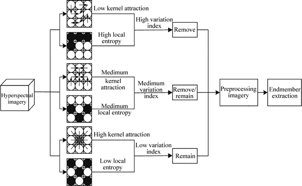
Fig. 3 Variation pixels identification technique
3 Experiments and results
The proposed method was conducted on two real hyperspectral data sets. Three classical endmember extraction methodologies (N-FINDR, VCA and OSP method) were employed to test the efficiency of the proposed method. What should be pointed out is that in this section we use capital O (data type O) to indicate the original data set. The capital P (data type P) denotes preprocessing data in which variation pixels have been removed.
3.1 AVIRIS Indian Pines scene data
The AVIRIS Indian Pines scene was collected in June 1992 with wavelength ranging from 0.4 to 2.5 ��m. After removing low SNR bands and high relative bands, 100 bands were selected from the original hyperspectral data cube. The spatial size for this data is 144��144. There are 16 distinct land-surface classes. Figure 4(a) shows 10th bands of this scene and Fig. 4(b) shows the ground-truth of 16 classes.
In this Indian pines scene, hundreds of pixels in the same block belong to the same category, but they show spectrum variability. Figure 5 exhibits 50 randomly selected spectral signatures of corn-notill corn-min, and corn, respectively. Spectral signatures vary around the mean spectral signatures. What is worse, corn-notill, corn-min and corn are spatial neighbors (Fig. 4) and similar species. This phenomenon brings a hard task for hyperspectral endmember extraction.
The proposed method was conducted on this data. Due to lack of prior knowledge, the threshold factor is ��=100%. Firstly, the number of endmembers D is evaluated by virtual dimension (VD) method [34]. When rf=10-3 (rf is the false alarm probability), D=18.
Figure 6 illustrates the endmember extraction results of corn-notill, corn-min and corn. Though corn- notill, corn-min and corn are three different land-surface classes, there are a large number of pixels coincided within the simplex. Obviously, variation pixels, particularly for corn-notill category, misguide estimation of the simplex volume. After removing variation pixels, the extracted endmembers close to centers of classes. There is a significantly improved results for VCA method (Fig. 6(b)).
Correspondingly, Fig. 7 compares the spectral angles between endmembers. The spectral angles (As) were calculated as
 (11)
(11)
where x and y are experimental and reference endmember vectors, respectively.

Fig. 4 AVIRIS Indian Pines Scene data:

Fig. 5 Spectral signatures of corn-notill (a), corn-min (b) and corn (c)

Fig. 6 Results of endmember extraction:
In Fig. 7, the solid lines indicate reference endmembers (mean of all samples), the dotted lines are endmembers extracted from original data set (data type O) and the dashed lines are endmembers extracted from preprocessing data set (data type P). The labeled numbers are spectral angles calculated by experimental endmembers and reference endmembers, where ��1 denotes the angle between endmembers extracted from original data and reference endmembers and ��2 denotes the angle between endmembers extracted from preprocessing data and reference endmembers. Obviously, the sum spectral angle of three endmembers is lower than original result. For N-FINDR method, the sum spectral angle is about 0.35, but for preprocessing data it is about 0.30. For VCA method, the spectral angle drops from 0.36 to 0.26. For OSP method, it decreases from 0.35 to 0.30.
The reconstitution RMSEs of 16 classes of this scene were compared, as shown in Table 1. The RMSE is calculated as follows
 (12)
(12)
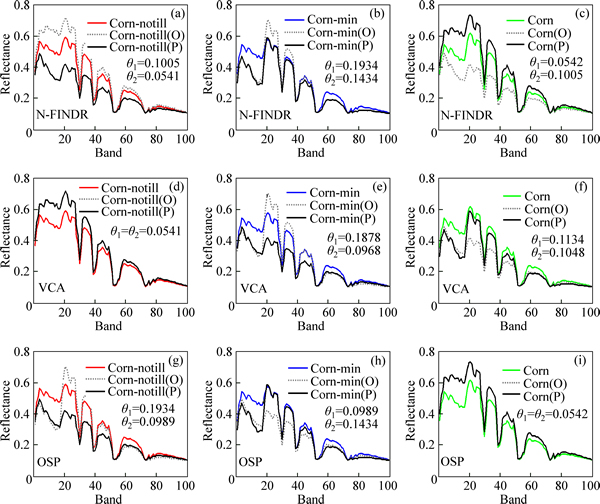
Fig. 7 Spectral angles of endmembers
Table 1 Comparison of RMSE

where  and
and  are respectively the reference value and reconstruction value of pixel ri,j related to category t of the k-th bands and U is the total number of samples of category t.
Obviously, the reconstitution RMSEs significantly decrease for most of the 16 land-surface classes after removing variation pixels. The average RMSE for N-FINDR method drops by about 10%, for VCA method it falls by around 25% and for OSP method it reduces by nearly 12%.
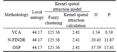
Table 2 shows the time consuming. This experiment was conducted on a computer equipment with 64 bits processor, CPU Intel Core i5, 2.60 GHz, RAM 4.00GB, matlab R2014a. Clearly, fuzzy clustering procedure consumes most of time, about 2 min. The cheerful results are that when dealing with data type P, the processing time for endmember extraction reduces by 62% for VCA, 33% for N-FINDR, 47% for OSP.
Table 2 Time consuming (Unit: s)
3.2 Salinas Valley scene data
The Salinas Valley scene was collected by AVIRIS sensor with 224 bands, spatial resolution 3.7 m. Bands of 108-112, 154-167 and 224 were removed due to water absorption. The complete data contain 16 land classes with spatial size 512��217. In this section, a subset of this data is adopted. This subset data comprise 86��83 pixels including 6 classes. Figure 8(a) shows the 120th band of Salinas scene and Fig. 8(b) shows 6 classes of this scene except the background.
Figure 9 compares the endmember extraction results (��=100%). To facilitate observation, the results with two mainly principal components axis for N-FINDR method and bands axis (band 35 and band 49) for VCA and OSP methods were presented. The extracted endmembers were labeled with black circles.
In Fig. 9, an apparent result is that there exist high variation pixels of class Brocoli_green_weeds_1, which are extracted as false endmembers for N-FINDR, VCA and OSP methods. Benefiting from the variation identification method, these high variation pixels are removed. Compared with original data set, the distribution of pixels in the simplex is more inerratic and partible. In Fig. 9(a), 3 classes (e.g. Brocoli_green_ weeds_1, Corn_senesced_green_weeds and Lettuce_ romaine_6wk) are extracted for N-FINDR method while for data type P, 5 classes are extracted. For VCA method (Fig. 9(b)), two more classes (Lettuce_romaine_4wk and Lettuce_romaine_6wk) are extracted compared with the original result. Specifically, four similar species (Lettuce_romaine_4wk, Lettuce_romaine_5wk, Lettuce_ romaine_6wk and Lettuce_romaine_7wk) are extracted accurately. For OSP method, Lettuce_romaine_4wk and Lettuce_romaine_5wk are distinguished exactly.
Figure 10 illustrates the relationship between the number of pixels removed and average RMSE and the threshold factor ��. There are totally 5348 pixels of these six classes. With the artificial threshold factor �� varying from 94% to 148%, the number of removed pixels ranging from 4802 to 0. Without any preprocessing (the points on the initial position), the average RMSE is 75.9 for N-FINDR method, 103.5 for VCA and 205.1 for OSP. When ��=120%, 83 pixels are removed. The average RMSE values go down sharply and remain a stable status, particularly for OSP and VCA method. Particularly, when ��=100% (Fig. 10(a)), 746 pixels were removed and the average RMSE is 32.6 for N-FINDR, 24.3 for VCA and 30.4 for OSP. The results indicate that 100% is a considerable value for �� without prior knowledge.
One key point should be noted that the value of �� is determined by the data inherent character. When modulating ��, the number of pixels remained should be higher than the minimum number of class samples.

Fig. 8 Salinas scene:
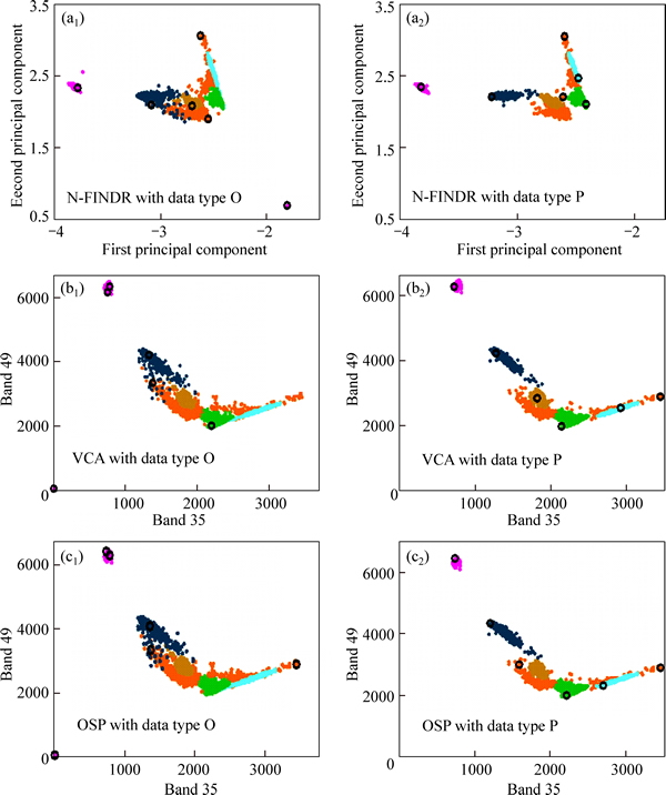
Fig. 9 Results of endmember extraction
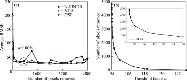
Fig. 10 Relationship between number of pixels removed and averge RMSE (a) and threshold factor �� (b)
4 Conclusions
1) Variation pixels interfere with the volume evaluation of a simplex. Some variation pixels essentially belong to the same category but extracted as distinct endmembers. The proposed variation pixels identification method is based on a kernel spatial attraction model and the local entropy theory. This method utilizes both spectral and spatial information with low computation complexity and understandable physical significance.
2) Specifically, to measure the degree of variability, the concept of variation index (VI) is defined. VI is proportional to local entropy while be inversely proportional to the kernel spatial attraction. Number of variation pixels to be removed is modulated by the threshold factor ��. Experimental results indicate that 100% is a considerable reference value for �� lack of prior knowledge.
3) The potential application of this method is that it can be used as a preprocessing procedure and combined with traditional geometric endmember extraction methods.
References
[1] CHANG C I. Hyperspectral data processing algorithm design and analysis [M]. USA, New York: John Wiley and Sons, 2013: 201-206.
[2] CHANG C I, PLAZA A. A fast iterative algorithm for implementation of pixel purity index [J]. Geoscience and Remote Sensing Letters, 2006, 3(1): 63-67.
[3] GRUNINGER J H, RATKOWSKI A J, HOKE M L. The sequential maximum angle convex cone (SMACC) endmember model [C]// Algorithms for Multispectral, Hyperspectral and Ultra-spectral Imagery. USA, Washington: SPIE, 2004: 3885-3895.
[4] HARSANYI J C, CHANG C I. Hyperspectral image classification and dimensionality reduction: An orthogonal subspace projection approach [J]. Geoscience and Remote Sensing, 1994, 32(4): 779-785.
[5] NASCIMENTO J M, BIOUCAS-DIAS J M. Vertex component analysis: A fast algorithm to unmix hyperspectral data [J]. Geoscience and Remote Sensing, 2005, 43(4): 898-910.
[6] WINTER M E. N-FINDR: An algorithm for fast autonomous spectral end-member determination in hyperspectral data [C]// Imaging Spectrometry V. Denver, USA: SPIE, 1999: 266-275.
[7] IORDACHE M D, BIOUCAS-DIAS J M, PLAZA A. Sparse unmixing of hyperspectral data [J]. Geoscience and Remote Sensing, 2011, 49(6): 2014-2039.
[8] MIAO Li-dan, QI Hai-rong. Endmember extraction from highly mixed data using minimum volume constrained nonnegative matrix factorization [J]. Geoscience and Remote Sensing, 2007, 45(3): 765-777.
[9] MOUSSAOUI S, HAUKSDOTTIR H, SCHMIDT F, JUTTEN C, CHANUSSOT J, BRIE D, DOUTE S. On the decomposition of Mars hyperspectral data by ICA and Bayesian positive source separation [J]. Neurocomputing, 2008, 71(10/11/12): 2194-2208.
[10] CHANG C I, WU C c, LO C s, CHANG M l. Real-time simplex growing algorithms for hyperspectral endmember extraction [J]. Geoscience and Remote Sensing, 2010, 48(4): 1834-1850.
[11] HEINZ D C, CHANG C I. Real-time processing of an unsupervised constrained linear spectral unmixing algorithm [C]// International Geoscience and Remote Sensing Symposium. Piscataway, USA: Institute of Electrical and Electronics Engineers Inc, 2001: 372-374.
[12] SOMERS B, ASNER G P, TITS L, COPPIN P. Endmember variability in spectral mixture analysis: A review [J]. Remote Sensing of Environment, 2011, 115(7): 1603-1616.
[13] KESHAVA N, MUSTARD J F. Spectral unmixing [J]. Signal Processing Magazine, 2002, 19(1): 44-57.
[14] CHANG C I, WU C c, LIU W m, OUYANG Y C. A new growing method for simplex-based endmember extraction algorithm [J]. Geoscience and Remote Sensing, 2006, 44(10): 2804-2819.
[15] PLAZA A, MARTINEZ P,  R, PLAZA J. Spatial/spectral endmember extraction by multidimensional morphological operations [J]. Geoscience and Remote Sensing, 2002, 40(9): 2025-2041.
[16] LIU Jun-ming, ZHANG Jiang-she. A new maximum simplex volume method based on householder transformation for endmember extraction [J]. IEEE Transaction on Geoscience and Remote Sensing, 2012, 50(1): 104-118.
[17] REZAEI Y, MOBASHERI M R, ZOEJ M J V, SCHAEPMAN M E. Endmember extraction using a combination of orthogonal projection and genetic algorithm [J]. Geoscience and Remote Sensing Letters, 2012, 9(2): 161-165.
[18] CHANG C I, WU C c, TSAI C T. Random N-Finder (N-FINDR) endmember extraction algorithms for hyperspectral imagery [J]. Image Processing, 2011, 20(3): 641-656.
[19] CALLICO G M, LOPEZ S, AGUILAR B, LOPEZ J F, SARMIENTO R. Parallel implementation of the modified vertex component analysis algorithm for hyperspectral unmixing using OpenCL [J]. Journal of Selected Topics in Applied Earth Observations and Remote Sensing, 2014, 7(8): 3650-3659.
[20] ZHANG J k, RIVARD B,  A, CASTRO- ESAU K. Intra-and inter-class spectral variability of tropical tree species at La Selva, Costa Rica: Implications for species identification using HYDICE imagery [J]. Remote Sensing of Environment, 2006, 105(2): 129-141.
[21] ZARE A, HO K C. Endmember variability in hyperspectral analysis: addressing spectral variability during spectral unmixing [J]. Signal Processing Magazine, 2014, 31(1): 95-104.
[22] ROBERTS D A, GARDNER M, CHURCH R, USTIN S, SCHEER G, GREEN R O. Mapping chaparral in the Santa Monica mountains using multiple endmember spectral mixture models [J]. Remote Sensing of Environment, 1998, 65(3): 267-279.
[23] ASNER G, BUSTAMANTE M, TOWNSEND A. Scale dependence of biophysical structure in deforested areas bordering the Tapajs national forest [J]. Remote Sensing of Environment, 2003, 87(4): 507-520.
[24] BATESON C A, ASNER G P, WESSMAN C A. Endmember bundles: A new approach to incorporating endmember variability into spectral mixture analysis [J]. Geoscience and Remote Sensing, 2000, 38(2): 1083-1093.
[25] JIN Jing, WANG Bin, ZHANG Li-ming. A novel approach based on fisher discriminant null space for decomposition of mixed pixels in hyperspectral imagery [J]. Geoscience and Remote Sensing Letters, 2010, 7(4): 699-703.
[26] MIANJI F A, ZHANG Y. SVM-based unmixing-to-classification conversion for hyperspectral abundance quantification [J]. Geoscience and Remote Sensing, 2011, 49(11): 4318-4327.
[27] CASTRODAD A, XING Z m, GREER J B, BOSCH E, CARIN L, SAPIRO G. Learning discriminative sparse representations for modeling, source separation, and mapping of hyperspectral imagery [J]. Geoscience and Remote Sensing, 2011, 49(11): 4263-4281.
[28]  G, PLAZA A. Spatial-spectral preprocessing prior to endmember identification and unmixing of remotely sensed hyperspectral data [J]. Journal of Selected Topics in Applied Earth Observations and Remote Sensing, 2012, 5(2): 380-395.
[29] ZORTEA M, PLAZA A. Spatial preprocessing for endmember extraction [J]. Geoscience and Remote Sensing, 2009, 47(8): 2679-2693.
[30] ZORTEA M, PLAZA A. Spatial-spectral endmember extraction from remotely sensed hyperspectral images using the watershed transformation [C]// Geoscience and Remote Sensing Symposium. Piscataway, USA: Institute of Electrical and Electronics Engineers Inc, 2010: 963-966.
[31] LOPEZ S, MOURE J F, PLAZA A, CALLICO G M, LOPEZ J F, SARMIENTO R. A new preprocessing technique for fast hyperspectral endmember extraction [J]. Geoscience and Remote Sensing Letters, 2013, 10(5): 1070-1074.
[32] MERTENS K C, BASETS B D, VERBEKE L P C, WULF R R D. A sub-pixel mapping algorithm based on sub-pixel/pixel spatial attraction models [J]. International Journal of Remote Sensing, 2006, 27(15): 3293-3310.
[33] BEZDEK J C. Cluster validity with fuzzy sets [J]. Journal of Cybernetics, 1973, 3(3): 58-73.
[34] CHANG C I, DU Q. Estimation of number of spectrally distinct signal sources in hyperspectral imagery [J]. Geoscience and Remote Sensing, 2004, 42(3): 608-619.
(Edited by FANG Jing-hua)
Foundation item: Projects(61571145, 61405041) supported by the National Natural Science Foundation of China; Project(2014M551221) supported by the China Postdoctoral Science Foundation, China; Project(LBH-Z13057) supported by the Heilongjiang Postdoctoral Science Found, China; Project(ZD201216) supported by the Key Program of Heilongjiang Natural Science Foundation, China; Project(RC2013XK009003) supported by the Program of Excellent Academic Leaders of Harbin, China; Project(HEUCF1508) supported by the Fundamental Research Funds for the Central Universities, China
Received date: 2015-04-14; Accepted date: 2015-09-24
Corresponding author: ZHAO Chun-hui, Professor, PhD; Tel: +86-18845870228; E-mail: zhaochunhui1965@126.com
Abstract: A variation pixels identification method was proposed aiming at depressing the effect of variation pixels, which dilates the theoretical hyperspectral data simplex and misguides volume evaluation of the simplex. With integration of both spatial and spectral information, this method quantitatively defines a variation index for every pixel. The variation index is proportional to pixels local entropy but inversely proportional to pixels kernel spatial attraction. The number of pixels removed was modulated by an artificial threshold factor ��. Two real hyperspectral data sets were employed to examine the endmember extraction results. The reconstruction errors of preprocessing data as opposed to the result of original data were compared. The experimental results show that the number of distinct endmembers extracted has increased and the reconstruction error is greatly reduced. 100% is an optional value for the threshold factor �� when dealing with no prior knowledge hyperspectral data.
