
LS-SVR method of ore grade estimation in Solwara 1 region with missing data
ZHANG Xu-nan(������)1, SONG Shi-ji(��ʿ��)1, LI Jia-biao(��ұ�)2, ZHOU Ning(����)3
(1. Department of Automation, Tsinghua University, Beijing 100084, China;
2. Second Institute of Oceanography, SOA, Hangzhou 310012, China;
3. China Ocean Mineral Resources R&D Association, Beijing 100860, China)
Abstract: Seafloor hydrothermal sulphide is a new poly metallic ore resource as well as oceanic poly metallic nodules and rich-Co crust containing huge amounts of metals and rare metals. The appropriate and accurate estimation of ore grade plays an important role for the prediction of total mineral resources and further exploitation. Kriging and neural network methods have already been successfully used for grade estimation problem. However, the performance of these methods is not perfect for the limited borehole data. Therefore, this paper introduces a new nonlinear method to the issue of ore grade estimation based on the least squares support vector regression (LS-SVR). The borehole data obtained from Solwara 1 region are heterogeneous and discontinuities with huge missing values. Data preprocessing methods including weighted K-nearest neighbor (WKNN) imputation and Genetic algorithm (GA) for data segmentation were used before using LS-SVR algorithm. Finally the performance and efficacy of the LS-SVR were compared with BP, RBF neural network and geostatistical techniques such as inverse distance weight (IDW) and ordinary kriging (OK). The outcome indicates that the LS-SVR method outperforms other four methods.
Key words: grade estimation; LS-SVR; missing data; WKNN; genetic algorithm
CLC number: P734 Document code: A Article ID: 1672-7207(2011)S2-0147-09
1 Introduction
Seafloor hydrothermal sulphide is a new poly metallic ore resource as well as oceanic poly metallic nodules and rich-Co crust, which contains huge amounts of metals and rare metals, such as Cu, Fe, Mn, Ag, Au, etc. The deposits are located at mid-ocean ridge, back-arc basin, island arc, sea mounts and so forth. Evaluation of an ore��s potential resource is utmost important for further decision and exploitation, in which grade estimation is actually one of the most key roles in mineral resources calculation[1].
The reliability of an ore grade model depends mainly on these three aspects: the first is the complexity and the spatial continuity of the ore body, the second is the reliability and adequacy of the data to capture the spatial variability, and the third is the type of used modeling technique[2]. During the past 30 years, geostatistics such as Kriging and its evolution methods have become popular ones which are widely used for grade estimation. They require certain assumptions such as the spatial distribution, priori knowledge and adequate data to be effectively applied. However, in most cases, the distribution of the ore is discontinuity and heterogeneous. High development cost and risk of drilling for the deep ocean work will restricts one to get adequate amount of exploratory borehole data, which cannot be collected as easily as on land. Recently, an alternative approach is the application of artificial neural networks (ANN) to grade estimation. ANN has good ability to solve complex and nonlinear problems, and it can easily capture nonlinear relationships between the input and output data. The application of different kinds of neural networks has been given by many researchers. Yama et al[3] developed a neural network model for learning the spatial continuity of a mineral field and, consequently, for predicting sulfur values for given coordinates. Samanta et al[4] applied different improved neural network model in a gold deposit and bauxite deposit which obtained better result compared to kriging and other techniques. Wu et al[5] used a multilayer feedforward neural network to capture the spatial distribution of ore grade. In addition, Samanta et al[6] solved the ore grade estimation problem based on the Wavelet Neural Network approach which offered a fast and robust estimation technique.
Although neural networks have played an important role in grade estimation, some shortcomings can not be neglected. First, a great amount of training data is needed in order to get a more accurate model. However, the borehole data got from deep sea are limited. Second, if the parameters are not chosen correctly, the generalization capability of ANN is not so well that over-fitting may occur. Besides, the ANN methods need much time to train the model even if they are better than traditional geostatistics. Due to these difficulties, this paper applies support vector regression (SVR) for grade estimation, which introduces Vapnik��s epsilon insensitive loss function in traditional support vector machines. The SVR embodies both the structural risk minimization (SRM) principle and empirical risk minimization (ERM) principle which has been shown to be superior to the conventional neural networks and classical statistical methods. Thus, it has excellent generalization capability to deal with limited sampling data. Moreover, the SVR formulation of the learning problem leads to quadratic programming with linear constraint, so it is easy to get the globally optimal solution avoiding getting local minima when using neural network methods. SVR has been successfully applied in many fields such as geology, meteorology, architectural structurology, etc[7-8]. In this paper, Least Square Support Vector Regression (LS-SVR) is used for solving the problem of ore grade estimation. It encompasses similar advantages as SVR, but requires solving a set of linear equations instead of quadratic programming, which is much easier and computationally simpler[9]. As the original borehole data in Solwara 1 Region are very heterogeneous and exist huge missing values, data preprocessing including weighted K-nearest neighbor (WKNN) imputation and genetic algorithm (GA) was given before the final grade estimation. WKNN is used to impute the missing data and GA is used to get reasonable data division for the training and testing data set.
2 Least square support vector regression algorithm
2.1 Basic support vector regression method
Burges[10] developed a novel machine learning method-SVM, which is based on VC dimension and structural risk minimization principle considering both training errors and generalization ability. SVM solves a constrained quadratic problem where the convex objective function for minimization given by the combination of a margin-based loss function with a regularization term. With the introduction of Vapnik��s ��-insensitive loss function, support vector regression (SVR) has been used to solve nonlinear regression estimation problems. Consider the problem of approximating the following dataset D={(x1, y1), ��, (xN, yN)}, x![]() Rn, y
Rn, y![]() R with a linear function:
R with a linear function:
![]() (1)
(1)
where w is the weights vector and b is the intercept that need to be estimated, and < , > denotes the dot product in X. The goal of SVR is to find a function f(x) that estimates the values of output variables with deviations less than or equal to �� from the actual training data, and at the same time is as flat as possible. The optimal regression function is determined by solving the following convex optimization problem:
 (2)
(2)
where ��i and ![]() are slack variables introduced to satisfy constraints and allow some errors. The regularization constant C>0 determines the trade-off between training error minimization and model complexity representing the ability of prediction for regression, and this penalty is acceptable only if the fitting error is larger than ��. This corresponds to dealing with a so called ��-insensitive loss function |��|�� described by
are slack variables introduced to satisfy constraints and allow some errors. The regularization constant C>0 determines the trade-off between training error minimization and model complexity representing the ability of prediction for regression, and this penalty is acceptable only if the fitting error is larger than ��. This corresponds to dealing with a so called ��-insensitive loss function |��|�� described by
![]() (3)
(3)
As depicted in Fig.1, the ��-insensitive loss function can reduce the noise and be visualized as a tube (slack variables ��i and ![]() equivalent to the approximation accuracy in training data. Only the points outside the shaded region contribute to the cost insofar, as the deviations are penalized in a linear fashion. The points lying on or outside the ��-bound of the decision function are support vectors. On the right, the ��-insensitive loss function is shown in which the slope is determined by C. The parameters C and �� are defined by users according to empirical analysis or some search space algorithms. The first term of Eq.(1) is the VC confidence interval whereas the second one is the empirical risk. Both terms limit the upper bound of the generalization error rather than limit the training error. This means that SVR fits a function to the given data by not only minimizing the training error but also by penalizing complex fitting functions. It strikes a balance between the structural risk and empirical risk minimization which leads to better generalization performance than neural network models.
equivalent to the approximation accuracy in training data. Only the points outside the shaded region contribute to the cost insofar, as the deviations are penalized in a linear fashion. The points lying on or outside the ��-bound of the decision function are support vectors. On the right, the ��-insensitive loss function is shown in which the slope is determined by C. The parameters C and �� are defined by users according to empirical analysis or some search space algorithms. The first term of Eq.(1) is the VC confidence interval whereas the second one is the empirical risk. Both terms limit the upper bound of the generalization error rather than limit the training error. This means that SVR fits a function to the given data by not only minimizing the training error but also by penalizing complex fitting functions. It strikes a balance between the structural risk and empirical risk minimization which leads to better generalization performance than neural network models.
It turns out that in most cases, the optimization problem given by the primal function can be solved more easily in its dual formulation. The key idea is to construct a Lagrangian function from the objective function and constraints by introducing a dual set of variables. The detailed deduction process can be found in Ref.[11].
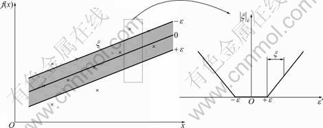
Fig.1 Soft margin loss setting for linear SVR
When solving nonlinear regression problem, we can map input training vectors x into vectors ��(x) of a higher dimensional feature space where the training data may be spread further apart and a larger margin may be found by performing linear regression in the new feature space. By introducing a kernel function K(xi, xw), it��s possible to calculate the dot product instead of actually mapping ��(x) into a higher feature space.
2.2 Least square support vector regression
Though the SVR method has a lot of advantages, it is solved using quadratic programming methods which are often time consuming and difficult to implement adaptively when the amount of data samples are huge. Hence, so as to reduce the complexity of optimization processes, a preferred version, called least square support vector regression (LS-SVR) is proposed, leading to solving a set of linear equations instead of solving a QP problem as in SVR. Meanwhile, it saves nearly the whole advantages of SVR.
Given a training data set of N points D={(x1, y1), ��, (xN, yN)}, x![]() Rn, y
Rn, y![]() R, the following regression model can be constructed by using nonlinear mapping function ��(��)
R, the following regression model can be constructed by using nonlinear mapping function ��(��)
![]() (4)
(4)
One considers the following optimization problem with an equality constraint-based formulation in primal space:
 (5)
(5)
where �� is the regularization parameter and ei is the error between actual output and predictive output of the i-th input data. The relative importance of these terms is determined by the positive real constant ��. In the case of noisy data one avoids overfitting by taking a smaller �� value. To solve the optimization problem (see Eq.(5)), the Lagrangian function is defined as:
![]() (6)
(6)
where ��i![]() R are Lagrange multipliers. The conditions for optimality are given by
R are Lagrange multipliers. The conditions for optimality are given by
 (7)
(7)
where i=1, ��, N. Then
![]() (8)
(8)
These conditions are similar to standard SVR optimality conditions, except for the condition ��i=ei. As a positive definite kernel ![]() is used, the prediction result f(x) could be evaluated as:
is used, the prediction result f(x) could be evaluated as:
![]() (9)
(9)
The parameter �� follows from solving a set of linear equations after elimination of w, e:
 (10)
(10)
with
![]()
and ![]() for i, w=1, ��, N. Then get the solution of �� and b. From Eq.(10), usually most of the Lagrange multipliers are support vectors not equal to zero, which means that the resulting network size is large and the solution is not as sparse as standard SVR. However, a sparse solution can be easily achieved via pruning or reduction techniques[12]. There are many kernel functions we can choose such as polynomial, radial basis function (RBF), sigmoid, etc. RBF used in this paper is as follows:
for i, w=1, ��, N. Then get the solution of �� and b. From Eq.(10), usually most of the Lagrange multipliers are support vectors not equal to zero, which means that the resulting network size is large and the solution is not as sparse as standard SVR. However, a sparse solution can be easily achieved via pruning or reduction techniques[12]. There are many kernel functions we can choose such as polynomial, radial basis function (RBF), sigmoid, etc. RBF used in this paper is as follows:
![]() (11)
(11)
3 Original data preprocessing for grade estimation
This study is conducted using drill-hole sampling data collected from Solwara 1 deposit region, which is situated in the Bismarck Sea within the New Ireland Province of PNG, at latitude 3.789��S, longitude 152.094��E. The site is about 50 km north of Rabaul and about 40 km west of Namatanai, occurring on a small ridge on the NW flank of the North Su volcanic center at depths of ~1 500 mBSL to ~1 700 mBSL (BSL means below sea level). The deposit is a stratabound zone of massive and semi-massive sulfide mineralization that occurs on a sub-sea volcanic mound which extends about 150 m to 200 m above the surrounding seafloor. The prospect contains a substantial resource of massive base metal sulfides, gold and silver. In 2007, Nautilus completed a 111 hole drilling program from the Wave Mercury using ROVs lowered onto the seabed. Drilling program was designed to test the inferred location of the deposit initially on a 50 m by 50 m grid, with subsequent infill to a 25 m by 25 m grid.
3.1 Data statistical analysis
The data set includes totally 1342 sampling data with the lithological information and different attribute grades (Cu, Au, Ag, etc.), while containing more than 40% missing values. Prior to using the LS-SVR method for grade estimation, statistical analyses of the sampling drill data are carried out in detail first, as for the mean and variance we often use. From the statistic results of coefficient of variation in Table 1, it can be observed that the grades are highly dispersed and some outliers exist which will have some influence on the construction of forecasting model.
Figure 2 presents the histogram plot of the sampling data which indicates that the distribution is neither normal nor lognormal except for Cu. The data set characteristically contains a large proportion of low-value samples with small proportion of high-value samples.
From the basic statistical analysis, there are two problems needed to be solved before using the LS-SVR method for grade estimation. One is to fill up the missing values occurring in the original data set because simply deleting will cause substantial biases, especially when missing data are not randomly distributed and the missing amount is huge. The other is how to partition the data to balance the training set and testing set in case random division will make all the high-value samples or no high-value fall into the testing set, thus the model will not learn the extreme value patterns and finally affect its generalization capability and predictive accuracy.
3.2 Weighted KNN for missing data imputation
In many cases the simple and common strategy to deal with absent values is ignoring them directly. However, several works have demonstrated that such deletion can introduce substantial biases, especially when missing data are not randomly distributed[13]. The Weighted K-nearest neighbors (WKNN) imputation method was given, which took the actual geology distribution into consideration. This method model the missing data estimation based on information available in the data set.
KNN imputation algorithm uses only similar cases with the incomplete pattern rather than the whole data set[14]. The nearest neighbors are found by minimizing a distance function. Given an pattern x by an n-dimensional input vector ![]() Moreover, the notation m is a vector of binary variables such that mi=1. If xi is missing, mi=0. And
Moreover, the notation m is a vector of binary variables such that mi=1. If xi is missing, mi=0. And ![]() represents the set of K nearest neighbors of x arranged in increasing order of chosen distance. There are two important items when using KNN algorithm, one is the distance measure and the other is how to estimate the missing value. Given two sample data xa and xb, heterogeneous Euclidean overlap metric (HEOM) distance function is used and the definition of the HEOM distance between them is:
represents the set of K nearest neighbors of x arranged in increasing order of chosen distance. There are two important items when using KNN algorithm, one is the distance measure and the other is how to estimate the missing value. Given two sample data xa and xb, heterogeneous Euclidean overlap metric (HEOM) distance function is used and the definition of the HEOM distance between them is:
![]() (12)
(12)
where di(xai, xbi) is the distance between xa and xb on its i-th attribute:
 (13)
(13)
where max(xi) and min(xi) are the maximum and minimum values observed from the training set, respectively. Once the K neighbors have been found, a replacement value for the missing attribute value can be estimated. In general, the missing value is obtained by mean estimation:
![]() (14)
(14)
When considering the actual borehole data distribution and the datum need to be estimated is continuous variable, we give weighted mean estimation method. The imputed value ![]() is obtained by the weighted mean value of its K nearest neighbors:
is obtained by the weighted mean value of its K nearest neighbors:
![]() (15)
(15)
where wk denotes the weight associated to the kth neighbor. The choice for wk is the inverse square of the distance:
![]() (16)
(16)
Table 1 Descriptive statistics of sampling borehole data
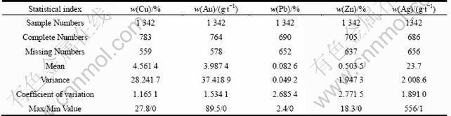
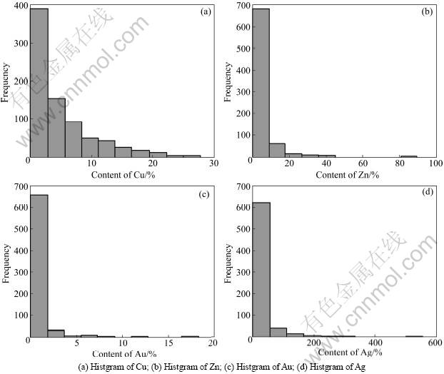
Fig.2 Histogram of different element attribute
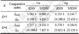
Cu and Ag were used as instances to certify the effectiveness of WKNN. The comparative experiment results between basic KNN and WKNN is shown in Table 2 with different choices of K. From the results of mean absolute error (IMAE) and error variance (IEV) it can be found that WKNN method mentioned above is better than KNN.
Table 2 Comparison results of basic KNN and WKNN method
3.3 Genetic algorithm for data division
In general, cross-validation method is used to train the model. However, in order to guarantee the generalization ability, we need to reasonably arrange the training data and testing data sets especially when the data used for grade estimation are exploratory borehole data. The pervious Fig.2 is the histogram of the borehole data, from which it can be found that the borehole data set are sparse and heterogeneous. It contains a large proportion of low-value samples with small proportion of high-value samples. Therefore, if the data set is divided randomly, some extreme high-value samples perhaps all fell into the testing data set so that the model parameters will be estimated inaccuracy. This will cause a problem of great errors in predicting the average grade value. Table 3 shows a simulation study about random selection algorithm of the data set. To eliminate the problem of large discrepancies in the mean and standard deviation values, genetic algorithm (GA) algorithm coupled with histogram-based data segmentation method to divide the borehole data set was introduced.
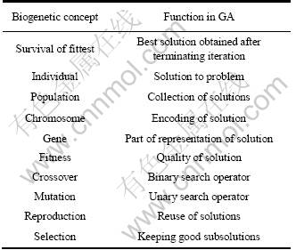
Genetic algorithms are one of the computational models based on genetics and natural selection in the evolutionary process[15]. GA has been successfully applied to problems that are difficult to solve using conventional techniques such as scheduling problems, traveling salesperson problem, network routing problems. GA is started with a set of solutions which encodes a potential solution to a specific problem on a simple chromosome-like data structure, and through selection, crossover and mutation a new solution (offspring) will be obtained, repeating these process until to find the best solution. Here, the better offspring is selected according to their fitness function values which show its high ability to survive. The corresponding relation between GA and biogenetic concepts is shown in Table 4.
Table 3 Summary statistics of Cu using random division
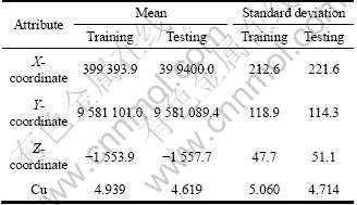
Table 4 Corresponding relation between GA and biogenetic concepts
Generally speaking, there are two main components of genetic algorithm that needs to be fixed before using it: the problem of encoding and the chosen of fitness function. We often seem the solution of one encodes as a chromosome, and the purpose of encoding is propitious to express the optimization problem and calculate the fitness function value. The fitness function is usually given as part of the problem description, and needs fast enough to compute. After making sure the fitness function, natural selection regularity is based on the value of each chromosome��s fitness function to decide which chromosomes are suit to be preserved. The general process of the genetic algorithm is as follows:
(1) Chromosome encoding of the original solution, setting the appropriate fitness function F(x) and stopping criteria.
(2) Randomly generate an initial source population of N chromosomes.
(3) Calculate the fitness F(x) of each chromosome x in the source population.
(4) Create an empty successor population and then repeat the following steps until N new chromosomes have been created.
![]() Reproduction: Roulette wheel of keeping better and discarding inferior chromosomes.
Reproduction: Roulette wheel of keeping better and discarding inferior chromosomes.
![]() Crossover: 1 1 1 0 0 0 | 1 0 | 0 1��1 1 1 0 0 0 | 0 1 | 1 0.
Crossover: 1 1 1 0 0 0 | 1 0 | 0 1��1 1 1 0 0 0 | 0 1 | 1 0.
![]() Mutation: 1 1 1 0 0 0 0 1 1 0��1 1 1 0 0 0 1 0 1 0.
Mutation: 1 1 1 0 0 0 0 1 1 0��1 1 1 0 0 0 1 0 1 0.
(5) Replace the source population with the successor population.
(6) Stop if stopping criteria have been met, else, return to(3).
In order to balance the training data and testing data set, each sample was encoded in training data set as binary coding 0 for testing notation and 1 for training notation. The fitness function is chosen as:
![]() (17)
(17)
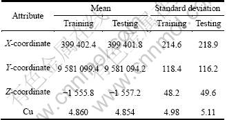
where m1, m2 and v1, v2 are the mean and variation values of training data and testing data respectively. However, there are some limitations. Therefore, during the process of crossover and mutation, one limitation needed to be added to keep the number of 0 and 1 is fixed. In order to get more accurate result, the data are firstly divided into reasonable parts consisting of low, medium, and high values according to the element content. Then, GA is used to each of these data sets. Table 5 presents the statistical properties of training data and testing data set for Cu element as obtained by using the mentioned technique of GA. From the comparison with Table 3, a more reasonable data division can be got for the final grade estimation by using GA method.
4 Grade estimation experiments in Solwara 1 region
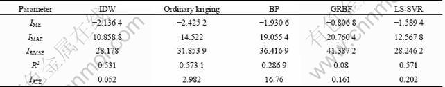
Using exploratory borehole data, the deposit was modeled by the LS-SVR method. There are totally 1342 borehole data with more than 40% missing values, WKNN method was used to imput the missing data, and then the complete dataset has been divided into two parts-training and testing dataset by using GA method. For construction the forecasting model, northing (Y), easting (X) and elevation (Z) coordinates were used as input variables and element contents as output variable. Various techniques such as Ordinary Kriging, IDW BP and Generalized RBF neural network were also investigated for comparison with LSSVR method. The performance analysis for all the models was tested on the same validation dataset. For comparison of these models, the following error statistics and efficiency index were used with y1 and y2 referring to actual and predicted values respectively.
Table 5 Summary statistics of Cu using GA division
(1) Mean error (ME):
![]()
(2) Mean absolute error (MAE)
![]()
(3) Root mean square error (RMSE):
![]()
(4) Coefficient of determination R2:
![]()
(5) Algorithm execution time (IAET).
The first two indicators show the accuracy and estimated ability of these models. The IRMSE takes into account both the bias and the error variance, and R2 represents the percentage of data variance explained by the model which signifies the predictive capacity of the model. Finally, the execution time shows the efficiency of these different models. Fig.3 gives the whole schematic diagram of the main steps that we mentioned above for grade estimation. A set of MATLAB codes were developed for the implementation of the algorithm.
Cu, Au, Zn, Pb and Ag are used as examples to illustrate the predicted comparison results, which were shown From Table 6 to Table 10. It can be seen apparently from the error statistics and efficiency index that IDW and LS-SVR have better performance than other models. Though IDW is faster than LS-SVR but later model has superior predictive capacity and generalization ability that is more suitable for the practical application.
5 Conclusions
In this study, the LS-SVR algorithm was investigated as a new modeling technique for grade estimation. Under the guarantee of statistical learning theory, LS-SVR has good generalization ability and execution efficiency to deal with small dataset, which solves the shortcomings existing in artificial neural network. As for the borehole data obtained from Solwara 1 region are not complete and are very heterogeneous containing a large proportion of low-value samples with small proportion of high-value samples. Weighted K-nearest neighbor (WKNN) imputation method was first applied to fill in the missing data. Genetic algorithm (GA) coupled with histogram-based data segmentation technique were then used to obtain reasonable training and testing data set so as to eliminate the large discrepancies caused by random data division. Finally the performance and efficacy of the LS-SVR method were tested against BP, RBF neural network and geostatistical techniques such as inverse distance weight (IDW) and ordinary kriging (OK). The outcome indicates that the LS-SVR model outperforms other methods.
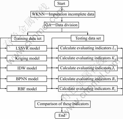
Fig.3 Schematic diagram of main steps for grade estimation in Solwara 1 region
Table 6 Comparative performance of different models for testing data set of Cu
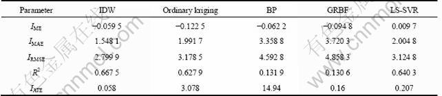
Table 7 Comparative performance of different models for testing data set of Au
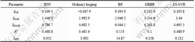
Table 8 Comparative performance of different models for testing data set of Pb
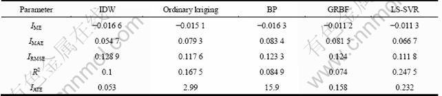
Table 9 Comparative performance of different models for testing data set of Zn
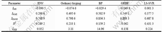
Table 10 Comparative performance of different models for testing data set of Ag
References
[1] Tutmez B. An uncertainty oriented fuzzy methodology for grade estimation[J]. Computers and Geosciences, 2007, 33(2): 280-288.
[2] Samanta B. Radial basis function network for ore grade estimation[J]. Natural Resources Research, 2010, 19(2): 91-102.
[3] Yama B R, Lineberry G T. Artificial neural network application for a predictive task in mining[J]. Mining Eng, 1999, 51(2): 59-64.
[4] Samanta B, Bandopadhyay S, Ganguli R, et al. Data segmentation and genetic algorithms for sparse data division in nome placer gold grade estimation using neural network and geostatistics[J]. Mining Explor Geol, 2002, 11(1-4): 69-76.
[5] Wu X, Zhou Y. Reserve estimation using neural network techniques[J]. Comput Geosci, 1993, 19(4): 567-575.
[6] Samanta B, Bandopadhyay S. Construction of a radial basis function network using an evolutionary algorithm for grade estimation in a placer gold deposit[J]. Computers & Geosciences, 2009, 35(8): 1592-1602.
[7] Anazi A F A L, Gates I D. Support vector regression for porosity prediction in a heterogeneous reservoir: A comparative study[J]. Computers & Geosciences, 2010, 36(2): 1494-1503.
[8] Rajasekaran S, Gayathri S, Lee T L. Support vector regression methodology for storm surge predictions[J]. Ocean Engineering, 2008, 35(16): 1578-1587.
[9] Suykens J A K, Vandewalle J. Least squares support vector machine classiers[J]. Neural Processing Letters, 1999, 9(3): 293-300.
[10] Burges C J C. A tutorial on support vector machines for pattern recognition[J]. Data Mining and Knowledge Discovery, 1998, 2: 121-167.
[11] Smola A J, Sch?lkopf B. A tutorial on support vector regression[J]. Statistics and Computing, 2004, 14(3): 199-222.
[12] Gencoglu M T, Uyar M. Prediction of flashover voltage of insulators using least squares support vector machines[J]. Expert Systems with Applications, 2009, 36: 10789-10798.
[13] Garc��a-Laencina P J, Sancho-G��mez J L, Figueiras-Vidal A R. Pattern classification with missing data: A review[J]. Neural Comput & Applic, 2010, 19(2): 263-282.
[14] Jerez J M, Molina I, Garc��a-Laencina P J, et al. Missing data imputation using statistical and machine learning methods in a real breast cancer problem[J]. Artificial Intelligence in Medicine, 2010, 50(2): 105-115.
[15] Chatterjee S, Laudatto M, Lunch L A. Genetic algorithms and their statistical applications: An introduction[J]. Computational Statistics & Data Analysis, 1996, 22(6): 633-651.
(Edited by DENG L��-xiang)
Received date: 2011-06-15; Accepted date: 2011-07-15
Foundation item: Project(60874071) supported by the National Natural Science Foundation of China; Project(DYXM-125-03-3) supported by the China Ocean Association; Projects(2009000, 2110035) supported by the Research Fund for the Doctoral Program of Higher Education; Project(2010THZ07002) supported by the Independent Research Project at Tsinghua University, China
Corresponding author: SONG Shi-ji; Tel: +86-10-62782721; E-mail: shijis@mail.tsinghua.edu.cn
