
Trans. Nonferrous Met. Soc. China 25(2015) 293-302
Three-dimensional analytical solution of acoustic emission source location for cuboid monitoring network without pre-measured wave velocity
Long-jun DONG1,2, Xi-bing LI1, Zi-long ZHOU1, Guang-hui CHEN1, Ju MA1
1. School of Resources and Safety Engineering, Central South University, Changsha 410083, China;
2. Australian Centre for Geomechanics, The University of Western Australia, Perth 6009, Australia
Received 27 August 2013; accepted 25 November 2014
Abstract:
To find analytical solutions of nonlinear systems for locating the acoustic emission/microseismic(AE/MS) source without knowing the wave velocity of structures, the sensor location coordinates were simplified as a cuboid monitoring network. Different locations of sensors on upper and lower surfaces were considered and used to establish nonlinear equations. Based on the proposed functions of time difference of arrivals, the analytical solutions were obtained using five sensors under three networks. The proposed analytical solutions were validated using authentic data of numerical tests and experiments. The results show that located results are consistent with authentic data, and the outstanding characteristics of the new solution are that the solved process is not influenced by the wave velocity knowledge and iterated algorithms.
Key words:
acoustic emission; seismic source; sensor; location; analytical solution;
1 Introduction
It is generally accepted that most solids emit low-level seismic signals when they are stressed or deformed. The solution of the problem of locating a signal source using time difference of arrival (TDOA) measurements has numerous applications in aerospace, surveillance, structural health, navigation, industrial process, speaker location, machine condition, monitoring of nuclear explosions, and mining induced areal seismology [1,2]. In the geotechnical field, this phenomenon is generally referred to as acoustic emission/microseismic (AE/MS) activities. When rock fractures, it produces AE/MS signals that transmit through the rock as elastic waves [3-5]. The application of the AE/MS system, which monitors self-generated acoustic signals occurring within the ground, has now rapidly increased for the monitoring of underground structures such as mines [6-8], tunnels [9-12], natural gas, nuclear engineering, and petroleum storage caverns, as well as surface structures such as foundations, rock, and soil slopes [13-16].
The location of a seismic event (earthquake, MS or AE) has been the first and most basic step in any study of seismicity on any scale since 1910 [17]. In general, earthquakes are predicted for their source locations, defined by the coordinates and the origin time, assuming a seismic velocity model and minimizing the difference between the observed and the calculated travel times. Source location is one of the classic problems in seismic areas [18,19]. Considerable number of studies published in the past more than 100 years on seismic source location have proved the importance and, at the same time, the complexity of this problem.
Many researchers have developed different AE/MS/seismic source location techniques, and some of which have been mature technologies and widely used in the positioning of AE/MS currently[20-23], for example the joint hypocenter determination method, the double- difference method, and topographic inverse [24-26]. Nevertheless, the problem of determining the four source parameters (geocentric: x, y, z and origin time) has still not be definitively solved. The iterative analytic procedures, which are nowadays most often used for the calculation (cf. Geiger��s method), are not infrequently divergent, or at any rate do not give very reliable results, which considerably reduces the number of well-located events. This can lead to negative consequences when interpreting the activity itself. It is well-known that the correct location of the source is dramatically hindered by the following factors: 1) insufficient knowledge of the seismic wave velocity; 2) inadequate distribution of the stations; 3) intrinsic limitations of the iteration algorithm applied. Generally, those factors do not act independently each other. Taking Geiger��s algorithm which is actually the widely used and known one as an example, the use of initial evaluated hypocenter coordinates is presupposed, and an iterative least-square technique is used. These conditions significantly influence the location accuracy.
DONG and LI [27] proposed a set of analytical solutions for the AE/MS source location under a cuboid monitoring network of sensor location. A location method with P-wave velocity by analytical solutions (P-VAS) was obtained with the established equations. Virtual location tests show that the relocation results of analytical method are fully consistent with the actual coordinates for events both inside and outside the monitoring network; whereas the location error of traditional time difference method is between 0.01 and 0.03 m for events inside the sensor array, and the location errors are large, which are up to 1080986 m for events outside the sensor arrays. The broken pencil location tests were carried out in a granite rock specimen with 350 mm in length and the cross section of 100 mm��98 mm, using five AE sensors. Five AE sources were relocated with the conventional method and the P-VAS method. For the four events outside monitoring network, the positioning accuracy by the P-VAS method is higher than that by the traditional method, and the location accuracy of the larger one can be increased by 17.61 mm. The results of both virtual and broken pencil location tests show that their resolved analytical solutions are effective to improve the positioning accuracy. However, the problem of the P-VAS is that the wave velocity should be given in advance. It is difficult to apply in the conditions without pre-measured velocity or pre-given velocity knowledge.
In this work, the analytical solutions of the AE/MS source location coordinates without the knowledge of wave velocity were developed. Different locations of sensors on upper and lower surfaces were considered and used to establish nonlinear equations. Based on the proposed functions of time difference of arrivals, the analytical solutions were obtained using five sensors under several networks without need of wave velocity. The method highlights three outstanding advantages: 1) without using iterative solution; 2) without initial evaluated hypocenter coordinates; 3) without pre- measured velocity or pre-given velocity knowledge.
2 Statement of problem and solution method
The AE/MS/seismic source location method using P-wave arrival time is widely used to calculate source coordinates for two reasons: the fastest propagation velocity, and the easy identification of first arrival time. The AE/MS/seismic source location coordinate is (x, y, z); Ti(i=1, 2, ��, n) is the ith monitoring station, and its coordinate is (xi, yi, zi) (i=1, 2, ��, n); li(i=1, 2, ��, n) is the distance from the AE/MS/seismic source to the station Ti; ti(i=1, 2, ��, n) is the arrival time recorded by sensor in the station Ti; t0 is the origin time of AE/MS source. Then, ti can be expressed as
 (1)
(1)
where  is the P-wave velocity.
By the spatial distance formula between two points (the source location and the monitoring station location), it can be obtained
 (2)
(2)
By taking Eq. (2) into Eq. (1), we have
 (3)
(3)
In Eq. (3), ti(i=1, 2, ��, n), v, and (xi, yi, zi) (i=1, 2, ��, n) are known; the seismic or AE source (x, y, z) and origin time  are unknown, which are needed to be solved. By taking each station data to Eq. (3), an equation can be obtained. Four stations correspond to four equations, and they can constitute a set of nonlinear equations. Generally, the greater the number of station is, the higher the positioning accuracy is. In the past more than 100 years, most researches were focused on the nonlinear optimization or iteration methods to locate the AE/MS/seismic source. The location precision was greatly influenced by the error of the wave velocity and the intrinsic limitations of the iteration algorithm applied. In this work, in order to find out the analytical solution of the AE/MS/seismic source location coordinates, the sensor location coordinates were optimized and simplified.
A cuboid monitoring network of sensor locations was selected, and the AE/MS/seismic source localization equations were established. The sensors are required to install at the vertices of the cuboid monitoring network. There are two cases including four sensors installed on one surface and additional one sensor on another surface (Fig. 1) as well as three sensors installed on one surface and additional two sensors on another surface (Fig. 2).
For every surface of the first case (Fig. 1), there are four types of monitoring network including Figs. 1(a), (b), (c) and (d). The first type (Fig. 1(a)) is analyzed in this work, and the others are similar. Five sensors are installed at vertices A, B, C, D and E of the cuboid monitoring network. The center of the cuboid is taken as the coordinate origin, and the coordinate direction is shown in Fig. 1.
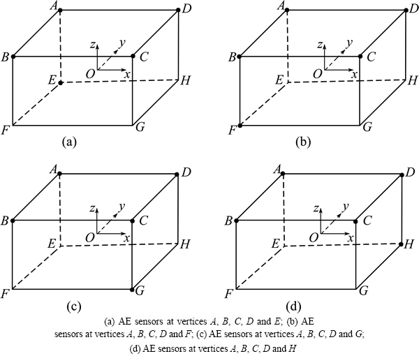
Fig. 1 Three-dimensional location schematic of cuboid monitoring network
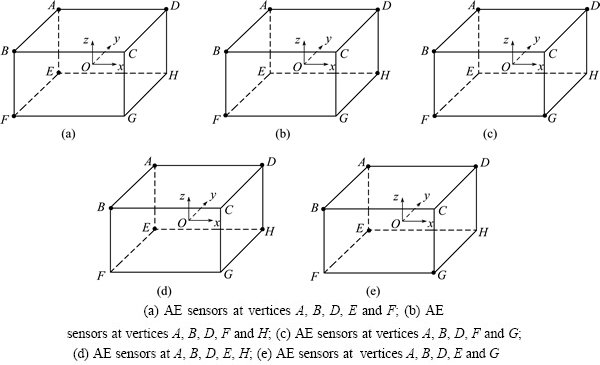
Fig. 2 Three-dimensional location schematic of cuboid monitoring network
The lengths of three sides of the monitoring network cuboid are 2a, 2b and 2c, respectively. The first sensor A is taken as a reference. The travel time of the sensor A from an AE/MS/seismic event is expressed as t10, and the arrival time of sensors B, C, D and E is t10+��t2, t10+��t3, t10+��t4, and t10+��t5, respectively. According to Eq. (3), it can be obtained
 (4)
(4)
 (5)
(5)
 (6)
(6)
 (7)
(7)
 (8)
(8)
Taking subtraction of Eqs.(4) and (5), Eqs. (4) and (6), Eqs. (4) and (7), as well as Eqs. (4) and (8), we have
 (9)
(9)
 (10)
(10)
 (11)
(11)
 (12)
(12)
From Eqs. (9) , (10) , and (11) one can easily obtain
 (13)
(13)
Resolving Eq. (13) yields
 (14)
(14)
Taking the ratio of Eq. (9) to Eq. (11), we have
 (15a)
(15a)
Supposing  , Eq. (15a) can be rewritten as
 (15b)
(15b)
From Eqs. (11) and (12) one can obtain
 (16)
(16)
Supposing , Eq. (16) can be rewritten as
 (17)
(17)
Eq. (4) divided by Eq. (9), we have
 (18)
(18)
Supposing  , and substituting Eqs. (15a) and (17) into Eq. (18), we have

 (19)
(19)
Eq. (19) can be rewritten as
 (20)
(20)
where

and C=a2+b2+c2+.
Then, x, y, and z can be obtained by resolving Eqs. (20), (15b) and (17). The solutions can be defined as analytical solution I (ASI).
For every surface of the second case in Fig. 2, there are five types of monitoring network including Figs. 2(a), (b), (c), (d) and (e). The first type (Fig. 2(a)) is analyzed in this work, and the others are similar. Five sensors are installed at vertices A, B, D, E, and F of the cuboid monitoring network. The center of the cuboid is taken as the coordinate origin, and the coordinate direction is shown in Fig. 2. The lengths of three sides of the monitoring network cuboid are 2as, 2bs and 2cs, respectively. The first sensor A is taken as a reference. The travel time from an AE/MS/seismic source (xs, ys, zs) to sensor A is expressed as ts10, and the arrival time of sensors B, D, E and F is ts10+��ts2, ts10+��ts3, ts10+��ts4 and ts10+��ts5, respectively. The P-wave velocity is expressed as vs. According to Eq. (3), it can be obtained
 (21)
(21)
 (22)
(22)
 (23)
(23)
 (24)
(24)
 (25)
(25)
Taking subtraction of Eqs. (21) and (22), Eqs. (21) and (23), Eqs. (21) and (24), as well as Eqs. (21) and (25), we have
 (26)
(26)
 (27)
(27)
 (28)
(28)
 (29)
(29)
From Eqs. (26), (28), and (29) one can easily obtain

 (30)
(30)
 (31)
(31)
From Eqs. (26) and (27) one can obtain
 (32)
(32)
Supposing  , Eq. (32) can be rewritten as
 (33)
(33)
From Eqs. (28) and (27) one can obtain
 (34)
(34)
Supposing  , Eq. (34) can be rewritten as
 (35)
(35)
From Eqs. (21) and (26) one can obtain
 (36)
(36)
Supposing  and substituting Eqs. (33) and (35) in Eq. (36), we have

 (37)
(37)
Equation (37) can be rewritten as
 (38)
(38)
where

and  . xs, ys, and zs can be obtained by resolving Eqs. (38), (33) and (35), respectively. The solutions can be defined as analytical solution II (ASII).
It is noted that the above two conditions are different networks which considered both upper and lower surfaces of the cuboid with five sensors. The first case is four sensors on upper surface and one sensor on the lower surface, while the second case is three sensors on upper surface and two sensors on the lower surface. The first case has four types of networks and the second one has five types of networks. It is easy to find the different and significant characteristics between the two types of networks. If we consider six surfaces of the cuboid networks, we can see that the two selected conditions have the same characteristic, four and one sensors on two different surfaces. It is noted that the condition that two and three sensors on two different surfaces is not considered. To fix the problem systematically, the third condition, two sensors on one surface and three sensors on another surface (Fig. 2(b)), is analyzed and the analytical solution is also obtained.
The lengths of three sides of the monitoring network cuboid are 2ap, 2bp and 2cp, respectively. The first sensor A is taken as a reference. The travel time from the AE/MS/seismic source (xp, yp, zp) to the sensor A is expressed as tp10, and the arrival time of sensors A, B, D, F and H is tp10+��tp2, tp10+��tp3, tp10+��tp4 and tp10+��tp5, respectively. The P-wave velocity is expressed as vp. According to Eq. (3), it can be obtained
 (39)
(39)
 (40)
(40)
 (41)
(41)
 (42)
(42)
 (43)
(43)
Taking subtraction of Eqs. (39) and (40), Eqs. (39) and (41), Eqs. (39) and (42), as well as Eqs. (39) and (43), we have
 (44)
(44)
 (45)
(45)
 (46)
(46)
 (47)
(47)
From Eqs. (44), (45), and (46) one can easily obtain

 (48)
(48)
 (49)
(49)
Taking the ratio of Eq. (44) and Eq. (45), we have
 (50)
(50)
Supposing  , Eq. (50) can be rewritten as
 (51)
(51)
Submitting Eq. (45) into Eq. (47) yields
 (52)
(52)
Taking the ratio of Eq. (52) and Eq. (45), we have
 (53)
(53)
Supposing  , Eq. (53) can be rewritten as
 (54)
(54)
Taking the ratio of Eq. (39) and Eq. (44) yields
 (55)
(55)
Supposing and substituting Eqs. (51) and (54) in Eq. (55), we have

 (56)
(56)
Eq. (56) can be rewritten as
 (57)
(57)
where


And
 .
.
xp, yp and zp can be obtained by resolving Eqs. (57), (51) and (54), respectively. The solutions can be defined as analytical solution III (ASIII).
3 Validated examples and discussion
3.1 Numerical examples
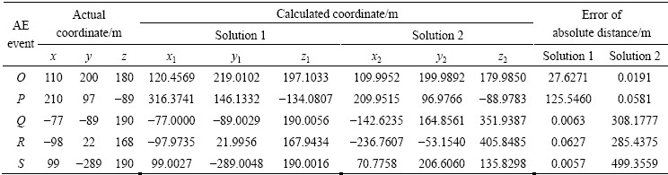
In the first example, a positioning system includes five sensors at the five cuboid vertices, and the coordinates are A(-130, 165, 220), B(-130, -165, 220), C(130, -165, 220), D(130, 165, 220), E(-130, 165, -220). The average equivalent P-wave velocity in the medium is expressed as v, and v=5000 m/s. The AE/MS sources are O(110, 200, 180), P(210, 97, -89), Q(-77, -89, 190), R(-98, 22, 168), and S(99, -289, 190) (all coordinates have the length unit of m). The arrival time recorded by sensors is listed in Table 1, and the accuracy of time is 10-6 s. By using the proposed analytical solution to calculate the AE/MS source coordinates, coordinate values of the five sensors and arrival time of five sensors for five events are taken into Eqs. (20), (15b) and (17), and the coordinate values (x, y, z) of five acoustic emission events can be resolved. The actual and calculated results are listed in Table 2. It can be seen from Table 2, one set of the location results of the proposed analytical solutions are fully consistent with the actual coordinates.
In the second example, a positioning system includes five sensors at the five cuboid vertices, and the coordinates are A(-130, 165, 220), B(-130, -165, 220), D(130, 165, 220), E (-130, 165, -220), and F(-130, -165, -220), and average equivalent P-wave velocity in the medium is expressed as v, and v=5000 m/s. Assume that AE/MS sources O, P, Q, R and S are as the same as the first example (all coordinates have the length unit of m). The arrival time recorded by sensors is listed in Table 3. By using the proposed analytical solution to calculate the AE/MS source coordinates, the coordinate values of the five sensors and arrival time of the five sensors for the five events are taken into Eqs. (38), (33) and (35), and the coordinate values (xs, ys, zs) of five acoustic emission events can be resolved. The actual and calculated results are listed in Table 4. It can be seen from Table 4 that one set of the location results of the proposed analytical solutions are fully consistent with the authentic coordinates.
Table 1 Arrival time recorded by sensors O, P, Q, R, and S in the first example
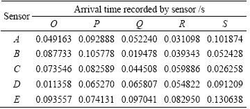
Table 2 Comparison between actual and calculated coordinates and errors of absolute distance in the first example
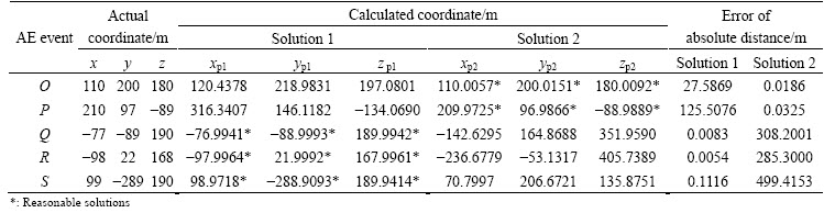
In the third example, a positioning system includes five sensors at the five cuboid vertices, and the coordinates are A(-130, 165, 220), B(-130, -165, 220), D(130, 165, 220), F (-130, -165, -220) and H(130, 165, -220). The average equivalent P-wave velocity in the medium is expressed as v, and v=5000 m/s. Assume that AE/MS sources O, P, Q, R and S are as the same as the first example (all coordinates have the length unit of m). The arrival time recorded by sensors is listed in Table 5. By using the proposed analytical solution to calculate the AE/MS source coordinates, the coordinate values (xp, yp, zp) of the five sensor and arrival time of five sensors for the five events are taken into equations (57), (51) and (54), and the coordinate values of the five acoustic emission events can be resolved. The actual and calculated results are listed in Table 6. It can be seen from Table 6 that one set of the location results of the proposed analytical solutions are fully consistent with the actual coordinates.
Table 3 Arrival time recorded by sensors A, B, D, E, and F in the second example
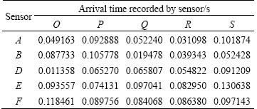
Table 4 Comparison between actual and calculated coordinates and errors of absolute distance in the second example
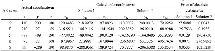
Table 5 Arrival time recorded by sensors in the third example
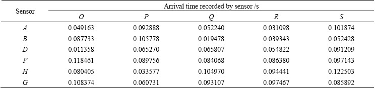
Table 6 Comparison between actual and calculated coordinates and errors of absolute distance in the third example
3.2 Experimental validation
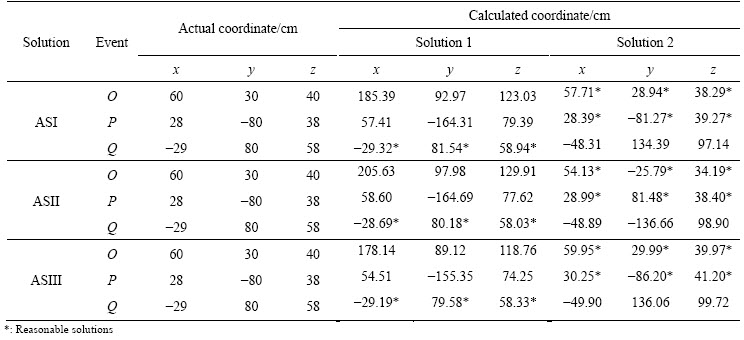
The AE tests were carried out in a cuboid of granite rock using five AE sensors. The sensor coordinates are A(-60, 80, 90), B(-60, -80, 90), C(60, -80, 90), D(60, 80, 90), E(-60, 80, -90). AE/MS sources are O(60, 30, 40), P(28, -80, 38) and Q (-29, 80, 58) (all coordinates have the length unit of cm). The arrival time recorded by sensors is listed in Table 7, and the accuracy of time is 10-6 s. By using the proposed analytical solution to calculate the AE/MS source coordinates, coordinate values of the five sensor and arrival time of the five sensors for five events are taken into equations of ASI, ASII and ASIII. The coordinate values of acoustic emission events can be resolved. The actual and calculated results are listed in Table 8. It can be seen from Table 8 that one set of the location results of the proposed analytical solutions are fully consistent with the actual coordinates.
It can be seen from the above validated examples that there are two groups of solutions using the proposed analytical solutions. One is the real and correct solution, the other one is meaningless solution. The problem is how to select the real solution and cancel the meaningless solution. The checking calculation with arrival time of the sixth sensor is an efficient approach to select a reasonable solution. For example, the arrival time of six sensors (i.e. sensor G) is listed in Table 5. The solutions in Table 6 are obtained only using the arrival time of the first five sensors. We can use arrival time tp6 and coordinates of the sixth sensor G to select the reasonable solution. The distance D between the solved source and sensor G can be calculated according to the distance formula between two points in space. vp can be solved using Eq. (39). According to tp10, the original time toriginal of the event can be obtained by taking the subtraction of tp1 and tp10, then the reasonable solution should meet the following criterion:
 (58)
(58)
Taking the values of sensor G into Eq. (58), we can easily get the reasonable solutions which are listed in Table 6.
Table 7 Arrival time recorded by sensors for three groups of AE tests
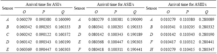
Table 8 Results and comparison of AE experiments
4 Conclusions
1) The sensor location coordinates were simplified as a cuboid monitoring network. Different locations of sensors on upper and lower surfaces were considered and used to establish nonlinear equations.
2) Based on the proposed functions of time difference of arrivals, the analytical solutions were obtained using five sensors under two networks. The proposed analytical solutions were validated using authentic data. The results show that the proposed analytical solution is reasonable and a set of the resolved solutions are consistent with the authentic results.
3) The sixth sensor is needed to determine the unique solution of the source location. Based on a cuboid monitoring network of sensor location, the method can locate the coordinates of AE/MS source only using simple four arithmetic operations. The method highlights three outstanding advantages of without using iterative solution, without initial evaluated hypocenter coordinates and without pre-measured velocity or pre-given velocity boundary conditions.
References
[1] ABDUL-WAHED M K, AL HEIB M, SENFAUTE G. Mining- induced seismicity: Seismic measurement using multiplet approach and numerical modeling [J]. Int J Coal Geol, 2006, 66(1-2): 137-147.
[2] DONG L J, LI X B, XIE G N. Nonlinear methodologies for identifying seismic event and nuclear explosion using random forest, support vector machine, and naive bayes classification [J]. Abstract and Applied Analysis, 2014, 2014: 459137.
[3] DONG L J, LI X B. A microseismic/acoustic emission source location method using arrival times of PS waves for unknown velocity system [J]. International Journal of Distributed Sensor Networks, 2013, 2013: 307489.
[4] LI X B, DONG L J. Comparison of two methods in acoustic emission source location using four sensors without measuring sonic speed [J]. Sensor Lett, 2011, 9(5): 2025-2029.
[5] DONG Long-jun, LI Xi-bing, TANG Li-zhong, Gong Feng-qiang. Mathematical functions and parameters for microseismic source location without pre-measuring speed [J]. Chinese Journal of Rock Mechanics and Engineering, 2011, 30(10): 2057-2067.(in Chinese)
[6] GE M. Source location error analysis and optimization methods [J]. Journal of Rock Mechanics and Geotechnical Engineering, 2012, 4(1): 1-10.
[7] DONG Long-jun, LI Xi-bing, PENG Kang. Prediction of rockburst classification using random Forest [J]. Transactions of Nonferrous Metals Society of China, 2013, 23(2): 472-477.
[8] CHEN B R, FENG X T, ZENG X, XIAO Y Y, ZHANG Z M, MING��J, WEI G L. Real-time microseismic monitoring and its characteristic analysis during TBM tunneling in deep-buried tunnel [J]. Chinese Journal of Rock Mechanics and Engineering, 2011, 30(2): 275-283. (in Chinese)
[9] CHENG Wu-wei, WANG Wen-you, HUANG Shi-qiang, MA Peng. Acoustic emission monitoring of TBM-excavated headrace tunnels of Jinping II hydropower station [J]. Journal of Rock Mechanics and Geotechnical Engineering, 2013, 5(6): 486-494.
[10] TANG Chun-an, WANG Ji-min, ZHANG Jing-jian. Preliminary engineering application of microseismic monitoring technique to rockburst prediction in tunneling of Jinping II project [J]. Journal of Rock Mechanics and Geotechnical Engineering, 2010, 2(3): 193-208.
[11] DONG L J, LI X B. Comprehensive models for evaluating rockmass stability based on statistical comparisons of multiple classifiers [J]. Mathematical Problems in Engineering, 2013, 2013: 395096.
[12] WANG Ji-min, ZENG Xiong-hui, ZHOU Ji-fang. Practices on rockburst prevention and control in headrace tunnels of Jinping II hydropower station [J]. Journal of Rock Mechanics and Geotechnical Engineering, 2012, 4(3): 258-268.
[13] DONG L J, LI X B, MA C D, ZHU W. Comparisons of Logistic regression and Fisher discriminant classifier to seismic event identification [J]. Disaster Advances, 2013, 6: s1-s8.
[14] LI X B, DONG L J, ZHAO G Y, HUANG M, LIU A H, ZENG L F, DONG L, CHEN G H. Stability analysis and comprehensive treatment methods of landslides under complex mining environment��A case study of Dahu landslide from Linbao Henan in China [J]. Safety Sci, 2012, 50(4): 695-704.
[15] DONG Long-jun, LI Xi-bing, ZHAO Guo-yan, GONG Feng-qiang. Fisher discriminant analysis model and its application to predicting destructive effect of masonry structure under blasting vibration of open-pit mine [J]. Chinese Journal of Rock Mechanics and Engineering, 2009, 28(4): 750-756. (in Chinese)
[16] DONG L J, LI X B, XU M, LI Q Y. Comparisons of random forest and support vector machine for predicting blasting vibration characteristic parameters [J]. Procedia Engineering, 2011, 26: 1772-1781.
[17] GEIGER L. Probability method for the determination of earthquake epicenters from the arrival time only [J]. Bulletin St Louis University, 1910, 8: 60-71.
[18] LI Qi-yue, DONG Long-jun, LI Xi-bing, YIN Zhi-qiang, LIU Xi-ling. Effects of sonic speed on location accuracy of acoustic emission source in rocks [J]. Transactions of Nonferrous Metals Society of China, 2011, 21(12): 2719-2726.
[19] LI X B, DONG L J. An efficient closed-form solution for acoustic emission source location in three-dimensional structures [J]. AIP Advances, 2014, 4(2): 027110.
[20] KUNDU T. Acoustic source localization [J]. Ultrasonics, 2014, 54 (1): 25�C38.
[21] CIAMPA F, MEO M, BARBIERI E. Impact localization in composite structures of arbitrary cross section [J]. Structural Health Monitoring, 2012, 11(6): 643�C655.
[22] NAKATANI H, KUNDU T, TAKEDA N. Improving accuracy of acoustic source localization in anisotropic plates [J]. Ultrasonics, 2014, 54(7): 1776-1778.
[23] PAVLIS G L. Appraising earthquake hypocenter location errors: A complete, practical approach for single-event locations [J]. Bulletin of the Seismological Society of America, 1986, 76(6): 1699-1717.
[24] PAVLIS G L, BOOKER J R. The mixed discrete-continuous inverse problem: Application to the simultaneous determination of earthquake hypocenters and velocity structure [J]. Journal of Geophysical Research, 1980, 85(B9): 4801-4810.
[25] WALDHAUSER F, ELLSWORTH W L. A double-difference earthquake location algorithm: Method and application to the northern Hayward fault, California [J]. Bulletin of the Seismological Society of America, 2000, 90(6): 1353-1368.
[26] DONG L J, LI X B, XIE G N. An analytical solution for acoustic emission source location for known P wave velocity system [J]. Mathematical Problems in Engineering, 2014, 2014: 290686.
[27] DONG Long-jun, LI Xi-bing. Three-dimensional analytical solution of acoustic emission or microseismic source location under cube monitoring network [J]. Transactions of Nonferrous Metals Society of China, 2012, 22(12): 3087-3094.
����Ԥ�Ȳ��ٵij�����������������Դ��ά������λ����
��¤��1,2, ��Ϧ��1, ������1, �¹��1, �� ��1
1. ���ϴ�ѧ ��Դ�밲ȫ����ѧԺ����ɳ 410083��
2. Australian Centre for Geomechanics, The University of Western Australia, Perth 6009, Australia
ժ Ҫ��Ϊ�õ�δ֪���ٽṹ������Դ��λ�������Ľ����⣬�����������м�Ϊ�����壬�������С��������µ�������Դ��λ�����⡣���Ǵ������ڳ�������治ͬλ�õĸ������Σ�������Ӧ�Ķ�λ���Ʒ����Է����顣���ݽ����ķ�����͵�ʱ�����������Ϊ3��������ֱ����δ֪��������²���5�����������ж�λ��������Դ��λ�����⡣���õ���������Դ��λ������Ӧ�õ���ֵ�������������н�����֤�������ʾ������õĽ����������Ԥ�Ȳⶨ����������㷨������λ����������λ�������ʵ����һ�¡�
�ؼ��ʣ������䣻��Դ������������λ��������
(Edited by Wei-ping CHEN)
Foundation item: Projects (11447242, 41272304, 51209236, 51274254) supported by the National Natural Science Foundation of China; Project (2015CB060200) supported by the National Basic Research Program of China
Corresponding author: Long-jun DONG; Tel: +86-13973160861; E-mail: rydong001@csu.edu.cn
DOI: 10.1016/S1003-6326(15)63604-4
Abstract: To find analytical solutions of nonlinear systems for locating the acoustic emission/microseismic(AE/MS) source without knowing the wave velocity of structures, the sensor location coordinates were simplified as a cuboid monitoring network. Different locations of sensors on upper and lower surfaces were considered and used to establish nonlinear equations. Based on the proposed functions of time difference of arrivals, the analytical solutions were obtained using five sensors under three networks. The proposed analytical solutions were validated using authentic data of numerical tests and experiments. The results show that located results are consistent with authentic data, and the outstanding characteristics of the new solution are that the solved process is not influenced by the wave velocity knowledge and iterated algorithms.
