
Determining simulation sample size for given precision requirements
SHI Peng(ʱ��), YANG Ming(����)
(Control and Simulation Centre, Harbin Institute of Technology, Harbin 150080, China)
Abstract: Simulation credibility evaluation concerns comparisons of the performance measures between simulation system and its reference counterpart. In fact, the required precision is known as prior information, which brings the problem of determining simulation run length according to the estimation of performance measures and the required precision. A feedback method was proposed from model analysis to data collection. For transient performance measures, operating characteristic curves were employed to calculate the simulation replications to detect the difference of means in parameter range. For steady-state performance measures, two phase method was put forward to satisfy the warm-up sizes at the first phase, and a run length for the relative- or absolute-precision requirement at the second phase. Some empirical experiments illustrate the validity of the proposed method.
Key words: simulation sample size; transient performance measures; steady-state performance measures; required precision; confidence interval
CLC number: TP391.9 Document code: A Article ID: 1672-7207(2011)S1-1114-05
The primary purpose of most simulation studies is the approximation of prescribed system parameters with the objective of identifying parameter values that optimize system performance measures[1]. Because of the stochastic input components of simulation models, its output is also random, so statistical technology should be used to analyze simulation results. Unfortunately, a simulation run does not usually produce independent and identically distributed (IID) observations, therefore, ��classical�� statistical techniques are not directly applicable to the analysis of simulation output. On the other hand, the precision required is always given as a criterion to judge whether the simulation system is credible and valid. Then the simulation sample size could be determined according to the estimation of parameters and required precisions.
There are primarily two types of performance measures for stochastic simulation systems: (1) transient performance measures, also known as terminating or finite-horizon measures, which evaluate the evolution of a system over a finite time horizon; (2) steady-state performance measures, also known as long-run or infinite-horizon measures[2], which describes how the system evolves over an infinite time horizon.
To determine the replications for transient measures, classical statistical techniques is applicable to analysis the simulation output, such as confidence interval for means. However, before the simulation execution, the resulting half width is not known how large, which depends on the output generated. The half width of confidence interval would be regardeel as the precision requirement, or the small pre-specified error. Nakayama[3] gave the sequential procedure to determine the run length, which contained generating trial run at first, regarding confidence interval as precision requirement approximately and computing the total sample size. Law et al[4-5] gave the procedure to construct confidence intervals for transient measures.
To determine the run length for steady-state measures, classical statistical techniques are not directly the output data from the simulations satisfied with the assumption of IID. normal, which has great impact on the estimation of steady-state measures. A procedure for determining whether these assumptions are satisfied is processed first. Chen et al[6-7] gave a procedure to check the independence and normality for the generaton of batch-means confidence intervals and proposed aquasi-independent procedure to determine the simulation run length. Calvin[7] gave an integrated paths method for simulation output analysis.
The main contribution of this work includes the following three points. First, simulation run length is calculated both for transient performance measures and steady-state performance measures. Second, precision requirement, variance estimation and Type II errors are taken into account for transient measures, making the analysis more realistic and credible. Third, warm-up sizes and precision requirement are considered together, bringing more accurate and credible results.
1 Output analysis for transient simulations
For transient simulation measure �� observations X1, X2, ������, Xn0, the small pre-specified error is ����. The mean and variance for �� are E(��) and ��X2, respectively, the sample mean is ![]() , the sample variance is S2(n), and the confidence interval for �� is
, the sample variance is S2(n), and the confidence interval for �� is ![]() , where n is the sample size,
, where n is the sample size, ![]() is the upper
is the upper ![]() quantile for normal distribution. Then the sample size required under the pre-specified error is
quantile for normal distribution. Then the sample size required under the pre-specified error is![]() .
.
There are two main problems in determining run length for transient measures: (1) the variance estimation in run length calculation based on half width of confidence interval is the approximate part sample variance estimation, which is bias from the real variance estimation; (2) Type II errors which are very important in simulation credibility evaluation are seldom considered. Two-stage method is proposed to determine the simulation sample size for transient simulation measures in requirement error range [B1, B2]. The main idea for two-stage method is that the confidence interval length decreases as the simulation sample size increases, until there is no significant difference between the values when �� = B1 , B2. Narrow the confidence interval (CI) until the difference is no longer significant, which means that the precision requirement is achieved, and the sample is in required simulation sample size. These two assumptions are listed below.
Assumption 1. The variances of the two samples �� = B1 and �� = B2 are approximate equal. That is Var[��] �֦�2, or Var[��] ��{Var[�� = B1]+ Var[�� = B2] }/2.
Assumption 2. The estimation E[��] is monotone in �� over [B1, B2]. This is a mild assumption, especially when the width of CI is small, indicating other values of �� in the entire range [B1, B2] are contained in the two values of B1 and B2.
��1 and ��2 are random variables depending on B1 and B2.
��1=E[��=B1]-{E[��=B1]+E[��=B2]}/2={E[��=B1]-E[��=B2]}/2.
��2=E[��=B2]-{E[��=B2]+E[��=B1]}/2={E[��=B2]-E[��=B1]}/2.
then the expectation of ![]() is an upper bound of the variability of the output.
is an upper bound of the variability of the output.
Theorem 1. X=[X1, X2,��, Xn]�� is the observation vector, ![]() is the sample mean of the observations, E[��] is the monotone in �� over [B1, B2], then is the upper bound for
is the sample mean of the observations, E[��] is the monotone in �� over [B1, B2], then is the upper bound for ![]() .
.
![]()
Algorithm 1. Two-stage procedure was selected to determine the simulation sample size for transient measures.
Step 1. Select n0, a sample size for the set of initial trial runs. Collect the output of �� = B1 and �� = B2, X11, X12, ������, X1n0 and X21, X22 , ������, X2n0;
Step 2. Calculate the sample means and variances ![]() ,
, ![]() , S1 and S2. S=(S1+S2)/2 is the approximate variance of �� over the range of [B1, B2];
, S1 and S2. S=(S1+S2)/2 is the approximate variance of �� over the range of [B1, B2];
Step 3. Calculate ![]() , where
, where ![]() is a measure of the difference in means against the sample variance;
is a measure of the difference in means against the sample variance;
Step 4. Calculate the sample size using the operating characteristic curves, and denote as Na according to the significant level ��, Type II error ��;
Step 5. Generate Na simulation samples, and collect the Na output sample values when �� = B1 and �� = B2. Then calculate![]() , and the required sample size Nb;
, and the required sample size Nb;
Step 6. Satisfy the sample size for the precision requirement N=Nb.
2 Output analysis for steady-state simulations
Common ways to determine the simulation run length for steady-state measures are mean estimation, variance estimation, confidence interval and pre-specified precision analogously to its transient counterpart. But there are some special characteristics in steady-state measures estimations, such as sample data are not IID, and there is autocorrelation, which makes a bias variance estimation and confidence interval; steady-state simulation systems could not replicate as many times as compared with the transient systems, and the initial transient bias should be considered.
2.1 Background
For steady-state simulation measure �� observations X1, X2,��, Xn0, the small pre-specified error is ����. The variance estimator S2(n) and confidence interval ![]() for �� used in transient simulations are not suitable in steady-state. The sample data are not IID and the autocorrelation and sample variance could not represent real parameter variance approximately. The required condition is that the autocorrelations of the stochastic process output die off as the lag among observations increases[8].
for �� used in transient simulations are not suitable in steady-state. The sample data are not IID and the autocorrelation and sample variance could not represent real parameter variance approximately. The required condition is that the autocorrelations of the stochastic process output die off as the lag among observations increases[8].
2.2 Batch means for IID samples
First, run the simulation system, and time series of the key parameter output data for each replication could be collected and represented by Yji, where i is the observation number and j is the replication number. Set the batch size k=1. The sample means at each observation can be calculated as:
![]() ,
,
where n is the number of replications performed. Vector ![]() represents the series of sample means, where m is the total number of observations in each replication.
represents the series of sample means, where m is the total number of observations in each replication.
Batch means are often used to obtain IID. normal data for steady-state simulation output results. A key problem using batch means method is the determinition of an appropriate batch size k. It is recommended that the run-length is doubled until the conditions for autocorrelation and normality are met. For instance, k0=5 is set initially, if the batch means are autocorrelation, k1 =10 would be tested. If this passes the procedure, k2 = 8 would be tested. If this fails to pass the procedure, k=10 would be the batch size. Then the smallest integer value of k could be found, when these batch means are approximately IID. Hence, the procedures could dynamically determine the appropriate batch sizes[9].
2.3 Run length for warm-up period
Steady-state simulation parameters could not get before system running, and the initial values would differ from the ones in steady-state. The most common method is transient bias selection and deletion method, such as statistical process control (SPC). The rules of SPC that identify the initial transient for a simulation with steady-state parameters are listed.
(1) A point plot outside a 3-sigma control limit;
(2) Nine consecutive points plot on one side of the mean;
(3) Six consecutive points plot increment or decrement;
(4) Fourteen consecutive points plot fluctuation;
(5) Two out of three consecutive points plot outside a 2-sigma control limit;
(6) Four out of five consecutive points plot outside a 1-sigma control limit;
(7) Initial points all plot to one side of the mean.
After that, the run length warm-up period N1 could be detected.
2.4 Run length for precision requirement
After the IID sample and initial transient deletion, the run length that satisfies the absolute or relative half-width requirements could be calculated. For steady-state simulation measure ��, batches observations X1, X2, ������, Xn0, the mean and variance for �� are E(��) and ��X2, respectively, the sample mean is ![]() , the sample variance is S2(n) and the confidence interval is
, the sample variance is S2(n) and the confidence interval is ![]()
![]() , where
, where ![]() is the
is the ![]() quantile for the N(0, 1) distribution and n is the sample size. Let the half width of the confidence interval
quantile for the N(0, 1) distribution and n is the sample size. Let the half width of the confidence interval ![]() . Next step is to determine whether CI meets the users�� requirements, and set �� and �� as the maximum absolute and relative half-width precision, respectively. That is
. Next step is to determine whether CI meets the users�� requirements, and set �� and �� as the maximum absolute and relative half-width precision, respectively. That is ![]() or
or ![]() , and the run length increases until the precision is satisfied.
, and the run length increases until the precision is satisfied.
The run length N2 under absolute precision �� is written as:
![]()
The run length N��2 under relative precision �� is written as:
![]() .
.
2.5 Compound run length for steady-state measures
Take the three aspecte into consideration, the procedure for calculating the run length of steady-state measures is obtained.
Algorithm 2. Two-stage procedure for steady-state measures to determine the simulation run length.
Step 1. Run the simulation system, perform replications and collect the output data.
Step 2. Set initial batch size k0 = 5, and calculate the batch means.
Step 3. If the batch means are not autocorrelations, go to step 4, otherwise increase the batch size until the batch means are i.i.d.
Step 4. If the batch number is lager than 20, go to step 5, otherwise increase the run length or the replications.
Step 5. Run length N1 for warm-up period would be go using the SPC method, and delete the initial bias data.
Step 6. If the mean estimations after initial bias deletion satisfy the precision requirements, go to step 7, or increase simulation replications.
Step 7. Calculate the run length N��2 under absolute precision �� and the run length N2�� under relative precision ��.
Step 8. The satisfied run length for the precision requirement is N=N1 +N2.
3 Empirical examples
3.1 Transient measures
Take a certain kind of launch precision in rail gun simulation system as an example[10]. Consider the velocity angle of the electromagnetic launch, the reference mean of which is 30��, precision error is ��0.5��, significant level ��=0.05 and Type II error is ��=0.1. Then the simulation sample size would be calculated to satisfy the precision requirements by Algorithm 1 in section 3.
Replicate N0=20 simulations at precision error range from 29.5 to 30.5, the means and variances of the two samples are (29.49, 20) and (30.50, 21), respectively. ![]() =0.012,
=0.012, ![]() ,
,
under ��=0.05 and ��=0.1, that indicates![]() , and the increase of the sample size is needed. Replicate Na=40 simulations at 29.5 and 30.5,
, and the increase of the sample size is needed. Replicate Na=40 simulations at 29.5 and 30.5, ![]() = 0.010, and
= 0.010, and![]() , under ��=0.05 and ��=0.1, that indicates n=35, and the decrease of the sample size is needed. Replicate Nb=30 simulations at 29.5 and 30.5,
, under ��=0.05 and ��=0.1, that indicates n=35, and the decrease of the sample size is needed. Replicate Nb=30 simulations at 29.5 and 30.5, ![]() =0.011,
=0.011, ![]()
![]() .
.

Fig.1 Procedure for simulation run length of steady-state measures
So, the simulation sample size is approximate 30, under the precision requirement of precision error ��0.5, significant level ��=0.05, and Type II error ��=0.1.
3.2 Steady-state measures
(1) Model 1, steady-state waiting-time process of M/M/1 queuing system. The arrival rate �� is set to 0.6 min, service rate �� is set to 1/min, that indicates ��=0.6, significant level ��=0.05, absolute precision ��=0.5, replication number is 100, run length is 500 and initial batch size k0 = 5.
(2) Model 2, steady-state waiting-time process of M/M/1 queuing system. The arrival rate �� is set to 0.8/ min, service rate �� is set to 1/min. Significant level ��=0.05, absolute precision ��=0.5, replication number is 100, run length is 500 and the initial batch size k0 = 5.
(3) Model 3, Steady-state waiting-time process of M/M/1 queuing system. The arrival rate �� is set to 0.9/ min, service rate �� is set to 1/min. Significant level ��=0.05, relative precision ��=3%, replication number is 100, run length is 800, and the initial batch size k0 = 5. The steady-state average waiting-time of the models is considered.
After the IID sample data are gotten, with batch size of 10, the warm-up period for the three models are 10, 90 and 250, respectively, as shown in Figs.2, 3 and 4. The left parts of these figures show the histogram of means and the right parts represent the relationship between batch means and control range. The horizontal ordinate is the sequence of batch means and the vertical ordinate depict the values of batch means. Tables 1 and 2 give the statistical results for state variables before and after initial bias data deletion, respectively.

Fig.2 SPC chart for Model 1

Fig.3 SPC chart for Model 2

Fig.4 SPC chart for Model 3
Table 1 Statistical results for state variables with no data deleted

Table 2 Statistical results for state variables after data are deleted
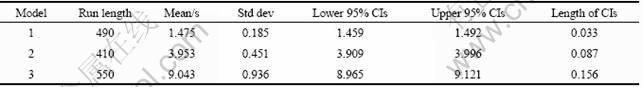
Table 3 Run length calculation for three models
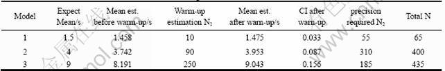
In the second stage, simulation run length that satisfies the precision requirements could be determined. The expected mean for the average waiting-time is 1.5, 4, and 9/min, respectively. Under the precision absolute requirements of 0.05, the requirement range for Model 1 is [1.45, 1.55]. Sample mean after initial data deletion falls in the range, the run length N2 that satisfies precision requirement is 55, and the total run length satisfies the users�� requirement is 65. Table 3 gives the run length calculation for the three models.
Empirical examples of the three queuing models show the efficiency of the proposed algorithm. Models 1 and 2 consider the absolute requirements and Model 3 depictes the relative requirements. The initial bias in Model 3 is lager, for the queue characteristics get worse as![]() .
.
4 Conclusions
(1) Two algorithms are presented to determine the simulation sample size for the given precision requirements. For transient performance measures, two phase method is put forward and operating characteristic curves are employed to calculate the simulation replications, which takes Type II error into consideration.
(2) For steady-state measures, another two phase method is proposed, which concerns the warm-up sizes at the first phase, and relative-or absolute-precision requirement at the second phase.
(3) In further researches, more attentions should be given in the areas with multivariable variable and proportional, quantile or derivative.
References
[1] Alexopoulos C, Kim S H. Review of advanced methods for simulation output analysis[C]// Proceedings of the Winter Simulation Conference. Orlando, US: Institute of Electrical and Electronics Engineers Inc. 2005: 188-201.
[2] Nakayama M K. Statistical analysis of simulation ouput[C]// Proceedings of the Winter Simulation Conference. Miami, US: Institute of Electrical and Electronics Engineers Inc. 2008: 62-72.
[3] Nakayama M K. Analysis of simulation output[C]// Proceedings of the Winter Simulation Conference. New Orleans, US: Institute of Electrical and Electronics Engineers Inc. 2003: 49-58.
[4] Law A M. Statistical analysis of simulation output data: the practical state of the art[C]// Proceedings of the 2004 Winter Simulation Conference. Washington D. S, US: Institute of Electrical and Electronics Engineers Inc. 2007: 67-72.
[5] Law A M. How to build valid and credible simulation model[C]// Proceeding of the 2009 Winter Simulation Conference. Austin, US: Institute of Electrical and Electronics Engineers Inc. 2009: 24-33.
[6] Chen E J, Kelton W D. A procedure for generating batch-means confidence intervals for simulation: Checking independence and normality[J]. simulation, 2007, 83(10): 683-694.
[7] Calvin J M. Simulation output analysis using integrated paths[J]. ACM Transactions on Modeling and Computer Simulation, 2007, 17(3): 1-24.
[8] Chen E J, Kelton W D. Determining simulation run length with the runs test[J]. Simulation Modelling Practice and Theory. 2003, 11(3): 237-250.
[9] Robinson S. A statistical process control approach to selecting a warm-up period for a discrete-event simulation[J]. European Journal of Operational Research. 2007, 176(1): 332-346.
[10] Min Fei-yan, Yang Ming, Wang Zi-cai. Critical problems of electromagnetic launch technique and its numerical simulation[J]. Journal of Solid Rocket Technology. 2009, 32(3): 237-241. (in Chinese)
(Edited by FANG Jing-hua)
Received date: 2011-04-15; Accepted date: 2011-06-15
Foundation item: Project (JC200606) Supported by the Foundation of the Outstanding Youth of Heilongjiang Province, China
Corresponding author: SHI Peng, PhD candidate; Tel: 13946026861; E-mail: shinkhit@yahoo.cn
