J. Cent. South Univ. Technol. (2011) 18: 1240-1247

DOI: 10.1007/s11771-011-0828-x

Calculation of earth pressure based on disturbed state concept theory

ZHU Jian-feng(朱剑锋)^{1, 2}, XU Ri-qing(徐日庆)², LI Xin-rui(李昕睿)², CHEN Ye-kai(陈页开)³

1. Faculty of Architectural Civil Engineering and Environment, Ningbo University, Ningbo 315211, China;

2. Key Laboratory of Soft Soils and Geoenvironmental Engineering, Ministry of Education,

Zhejiang University, Hangzhou 310058, China;

3. School of Civil Engineering and Transportation, South China University of Technology, Guangzhou 510640, China

? Central South University Press and Springer-Verlag Berlin Heidelberg 2011

Abstract: The theoretical formulations of Coulomb and Rankine still remain as the fundamental approaches to the analysis of most gravity-type retaining wall, with the assumption that sufficient lateral yield will occur to mobilize fully limited conditions behind the wall. The effects of the magnitude of wall movements and different wall-movement modes are not taken into consideration. The disturbance of backfill is considered to be related to the wall movement under translation mode. On the basis of disturbed state concept (DSC), a general disturbance function was proposed which ranged from -1 to 1. The disturbance variables could be determined from the measured wall movements. A novel approach that related to disturbed degree and the mobilized internal frictional angle of the backfill was also derived. A calculation method benefited from Rankine’s theory and the proposed approach was established to predict the magnitude and distribution of earth pressure from the cohesionless backfill under translation mode. The predicted results, including the magnitude and distribution of earth pressure, show good agreement with those of the model test and the finite element method. In addition, the disturbance parameter b was also discussed.

Key words: disturbed state concept; disturbance function; translation mode; earth pressure; cohesionless soil

1 Introduction

Retaining walls are mainly designed to resist lateral earth pressures. Traditionally, the forces acting on the wall are typically determined by using the Rankine and Coulomb’s theories of earth pressure and both theories assume the backfill to reach the limited equilibrium state. However, in most cases, the backfill is not in the limit condition. Valuable experimental and numerical simulation works on earth pressure against retaining wall had been conducted by many researchers [1-7]. It was found that the model and magnitude of wall movements had a great influence on the lateral earth pressures against the rigid retaining wall. Thus, it is essential to establish a calculation method under the consideration of wall-movement effect to predict the actual earth pressure.

In reality, the movement of a rigid retaining will disturb the backfill. Furthermore, the disturbance will change the strength parameters such as internal frictional angle (φ). The disturbance of soil can be evaluated by disturbed degree (D), which reflects the change of physical and mechanical parameters of the soil. It is impossible to predict the magnitude and distribution of lateral earth pressure against the wall during the disturbance process by Rankine or Coulomb’s theory. However, it could be possible to define the change in φ to be related to the wall movement (S), and thereby define the magnitude and distribution of lateral earth pressure as functions of φ. Such a procedure is possible through utilizing the disturbed sate concept (DSC) [8] which can provide micromechanical understanding of the problem. The DSC is a unified approach for constitutive modeling of the materials and interfaces, and is presented in a number of publications together with its applications to a wide range of materials such as clays, sands, porous saturated materials, and reinforced soil wall [9-12].

In the DSC, a deforming material element was treated as a mixture of the initial continuum or relative intact (RI) part and the fully adjusted (FA) part. The observed behavior of the material was expressed in terms of the coupled behavior of the materials in the RI and FA states by utilizing the disturbance function, D, which acted an interpolation and coupling mechanism between the RI and FA states. The disturbance could represent the effect of microcracking and fracture leading to degradation in which the value of D ranged from 0 to 1, and enhanced particle bonding leading to stiffening in which the value of D ranged from -1 to 0. Unfortunately, most disturbance functions proposed by Desai only considered the degradation effects with correspondent value of D ranging from 0 to 1. To date, general disturbance functions which can reflect the two effects of disturbance (damage and stiffening) have seldom been reported in the literature. Based on these characteristics, the main purposes of this work are summarized as follows:

1) Based on the DSC, a unified disturbance function was formulated for characterizing the disturbance of cohesionless backfill in translation mode. In this function, the disturbed degree (D) could range from -1 to 1.

2) A novel approach that related to the disturbed degree and the mobilized internal frictional angle of the backfill was also derived.

3) On the basis of the proposed approach, a calculation method benefited from Rankine’s theory was established to predict the actual magnitude and distribution of earth pressure.

4) A general discussion on the disturbance parameter b was made and additionally the acquisition region of b was given.

2 General disturbance function

Herein, it was supposed that the orientation of a rigid retaining wall moving toward backfill is positive. Then, the RI state can be considered to be such a state at which the rigid retaining wall moves toward or away from the backfill at a certain value (S₀), and S₀ can be negative, positive or zero. In most cases, the at-rest state is assumed to be the RI state, and the correspondent value of S₀ is zero. When the amount of wall movement approaches to a certain value (S_a or S_p), the backfill will reach the limited equilibrium state. So, the limit state can be considered as the FA state. According to Rankine’s theory, there are mainly two states, namely the active and passive Rankine state [13]. The amount of movement required to reach active Rankine state can be defined as S_a which is negative according to the positive orientation defined above. Then, the amount of movement that is needed to reach passive Rankine state can be defined as S_p with the correspondent value being positive.

2.1 Disturbance function

The disturbance function, D, is expressed as the ratio of the material volume in the FA state to the total volume of the material element [14]. Disturbance is considered to be affected by internal microstructural changes which could be defined by using such internal variable as the plastic strain (ε), as shown in Fig.1, e.g.,

                      (1)

where D_u, A, and Z are material parameters.

2.2 General disturbance function

There are a number of ways to define D as explained by DESAI [15]; unfortunately, most of them are proposed just taking into consideration of the disadvantageous disturbance (such as damaging materials) and their correspondent values of D only range from 0 to 1. However, the disturbance also includes the advantageous aspects (such as stiffening materials) in which the correspondent values of D may range from -1 to 0.

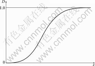
Fig.1 Relationship between disturbed degree and strain [14]

In addition, due to the fact the S is the integral of strain (ε), the relationship between D and rigid wall movement (S) can be supposed to be similar to that shown in Fig.1. Herein, defining that the value of D ranging from -1 to 0 and 0 to 1 as “negative disturbance” and “positive disturbance”, respectively, and considering that the limit condition of backfill includes two states, the general disturbance function can be defined as

For “positive disturbance”:

                                (2a)

For “negative disturbance”:

                                (2b)

where S denotes the current amount of the rigid wall movement; S₀ denotes the amount of the rigid wall movement at rest state which is generally set as zero; S_a denotes the amount of the rigid wall movement at active Rankine state which can range from -0.003H to -0.001H [16] (H is the total height of the retaining wall); S_p denotes the amount of the rigid wall movement at passive Rankine state which can range from 0.02H to 0.05H [16]; b denotes the disturbance parameter which is introduced to express the disturbance velocity of backfill. Meanwhile, b is related to the relative density of backfill.

According to the positive orientation defined above, the value of S_a and S_p are negative and positive, respectively.

The disturbance function is termed to be general because it allows for various states of backfill with the same mathematical framework. As shown in Fig.2, at first, the backfill is in at-rest state and there is no translation of the vertical rigid retaining wall, so the disturbance is zero. As the wall moves away from the backfill, the amount of movement (S) will decrease whereas the correspondent disturbed degree (D) will increase. When S approaches to S_a, D reaches 1 and the backfill achieves active Rankine state. As the wall moves toward the backfill, the amount of movement (S) will increase whereas the correspondent D will decrease. When S approaches to S_p, D reaches -1 and the backfill achieves passive Rankine state.

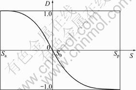
Fig.2 Relationship between disturbed degree and wall movement

3 Calculation of earth pressure based on DSC

The first step in the present analysis is to consider the case of a simple retaining wall, where 1) the backfill has a horizontal surface, 2) the face of the retaining wall in contact with the soil is vertical, and 3) there is no shear stress between the vertical face of the retaining wall and the soil, as shown in Fig.3.

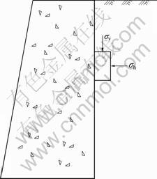
Fig.3 Schematic diagram of simple retaining wall

Suppose that such a soil deposit is stretched in the horizontal direction. Any element of soil behaves like a specimen of a triaxial test in which the confining stress is decreased or increased while the axial stress remains constant. At first, there is no wall movement, so the backfill is in at-rest state. The horizontal stress for this condition is called at-rest stress, and the ratio of horizontal to vertical stress is called the coefficient of at-rest stress and is denoted by the symbol K₀. For loose and medium dense cohesionless backfill, it can be expressed as [13]

                                                   (3)

Next, if the rigid wall moves away from the backfill, the disturbed degree (0h) of the soil element will reduce and the vertical stress (σ_v) will remain constant, as shown by the stress path (A→C) in Fig.4. When D approaches to 1, the horizontal stress will decrease to a certain magnitude in which the shear strength of the soil will be fully mobilized. No further decrease in σ_h is possible. The horizontal stress for this condition is called the active stress, and the ratio of horizontal to vertical stress is called the coefficient of active stress which can be denoted by the symbol K_a. The state of the active stress is called active Rankine state. Figure 5 shows the Mohr circle for the active state of stress. According to the Mohr-Coulomb failure law, the coefficient of the active stress can be defined as

                           (4)

where σ_h denotes the horizontal stress at active Rankine state; φ denotes the internal friction angle.

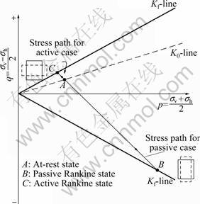
Fig.4 Stress paths for different conditions

Then, if the rigid wall moves toward the backfill, the disturbed degree (-1≤D<0) of the backfill will decrease, σ_h of the soil element will increase and σ_v will remain constant, as shown by the stress path (A→B) in Fig.4. When σ_h is increased up to σ_v, the Mohr circle for this condition is reduced to one point E, as shown in  Fig.5. The soil element is under the condition of isotropic compression. If the wall further moves toward the backfill, D will keep on decreasing, whereas σ_h will continue to increase. However, the horizontal stress cannot increase beyond a certain magnitude called the passive stress. In this case, the disturbed degree of backfill is -1. The ratio of horizontal to vertical stress is called the coefficient K_p of passive stress. The state of the passive stress is called passive Rankine state. Figure 5 also shows the Mohr circle for this state of stress, and the magnitude of K_p can be given by

                 (5)

where σ_h denotes the horizontal stress at passive Rankine state. Thus, for a given vertical geostatic stress σ_v, the horizontal stress can be only between the limits K_aσ_v and K_pσ_v.

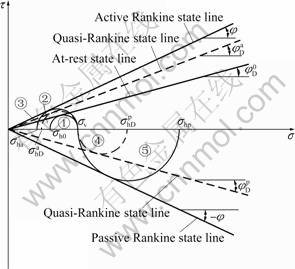
Fig.5 Horizontal stress at different disturbed states: ① At-rest state (D=0) and σ_h0=k₀σ_v; ② Quasi-Rankine state (0 ③ Active Rankine state (D=1) and σ_hD=k_aσ_v;④ Quasi-Rankine state (-1⑤ Passive Rankine state (D=-1) and σ_hp=k_pσ_v; E: Condition of isotropic compression and σ_h=σ_v

Suppose that the arbitrarily disturbed state between the active and passive Rankine state is in quasi-Rankine state. As shown in Fig.5,  and  denote the horizontal stress at the quasi-Rankine state with D being positive and negative, respectively. In this case, the friction angle can be denoted by the symbol φ_D, which must satisfy the following conditions:

For at-rest state,

                 (6a)

where  denotes the friction angle in at-rest state.

For active Rankine state,

φ_D=φ                                                (6b)

For passive Rankine state,

φ_D=-φ                                               (6c)

Since φ_D is related to the disturbance of backfill, it can be expressed as a function of D, as shown in Fig.6.

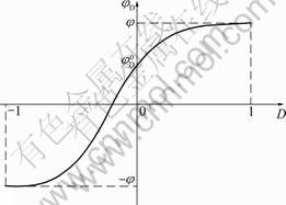
Fig.6 Relationship between disturbed degree and φ_D

Considering above conditions that φ_D must satisfy, a formula for φ_D can be derived as

                   (7)

Referring to Rankine’s theory, the coefficient (K_D) of lateral earth pressure at the quasi-Rankine state is

                         (8)

Hence, the lateral pressure (p_D) against a vertical rigid retaining wall can be

p_D=γhK_D                                        (9)

where γ is the unit weight of the backfill, h is the height of the calculated point and h ranges from 0 to H, and H is the total height of the retaining wall.

From above analysis, it can be seen that, once the parameters S, S_a, S_p, b, φ, γ and h are given, the magnitude and distribution of earth pressure can be predicted by the proposed calculation method.

4 Example and discussion

4.1 Example 1

The model wall was a 940 mm-wide, 1 000 mm- high, and 120 mm-thick solid plate, which was made of reinforced concrete. To investigate the distribution of earth pressure, thirteen soil pressure transducers were attached to the model retaining wall, as shown in Fig.7. Ten YB-1 mini-type earth pressure transducers had been arranged within the central zone of the wall. Another three transducers (SPT10, SPT11, SPT12) had been mounted between the central zone and sidewall to investigate the sidewall effect. Air-dry sand of Qiantang River of Hangzhou in China was used in this investigation. Physical properties of the soil include γ_d=15.462 kN/cm³, D_r=0.502, where γ_d and D_r denoted the in-place dry density, dry unit weight and relative density, respectively. Through direct shear test, the internal friction angle φ was 34.2° [7].

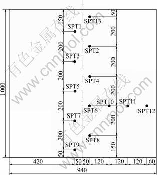
Fig.7 Location of earth pressure transducers (Unit: mm)

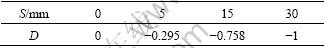
According to the test data, when the backfill reached passive Rankine state, the correspondent movement (S_p) of the rigid retaining wall was 0.03H (S_p=30 mm, for H= 1 000 mm). Since the test was mainly done for studying the passive earth pressure, the amount of movement S_a, which was needed to approach to active Rankine state, was not given in the model test. According to the results of numerical analyses, S_a could be taken to be -0.001 6H (S_a=-1.6 mm) [18]. The value of parameter b could be taken as 2.5 temporarily and the wall movement (S) in field could be obtained from the test data. Then, put the value of S, S_a, S_p and b into Eq.(2), the disturbed degree for each case could be calculated, as shown in Table 1.

Table 1 Disturbed degree of backfill

By utilizing the calculated value of D (Table 1) and Eq.(8) and Eq.(9), the lateral earth pressures predicted at different depths are shown in Fig.8. The variation of measured lateral earth pressures under different disturbed degrees is also shown in Fig.8.

As illustrated in Fig.8, the lateral earth pressure increases whereas the disturbed degree decreases. When D approaches to -1, the backfill reaches passive Rankine state. Then, the predicted distribution of earth pressure coincides with that of passive Rankine state. It can also be seen that the measured distribution of earth pressure along the depth is almost linear at different disturbed states, which means that the disturbance of the backfill along the depth is almost uniform for translation mode. The difference between the measured and predicted earth pressures is little. Moreover, the distribution of the predicted earth pressures agrees well with that of the measured values.

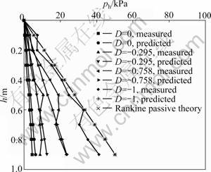
Fig.8 Distribution of lateral earth pressure under different disturbed degrees

4.2 Discussion on parameter b

As observed from Eq.(2), the absolute value of D approaches to 1 with increasing or decreasing the amount of movement. The rate of approach is mainly dependent on the value of parameter b. Its value was taken as 2.5 in the previous analyses. Now, five conditions in which the amount of wall movement (S) equaled 5, 10, 15, 20 and 25 mm were considered, respectively. Then, the relationship between b and D for each case is shown in Fig.9. It can be seen that, when b ranges from 0 to 0.5, the disturbed degree is quite sensitive to b. Therefore, it will give rise to great errors in computing disturbed degree of backfill by using the value of b in this region. When b is greater than 5, the D for each case will achieve a constant value, which can not be coincided with the practical situation. When b lies between 0.5 and 5, the variation of curves will become slow. The difference in the disturbed degree for different cases will agree well with the actual situation. Therefore, the parameter b can be chosen between 0.5 and 5.

In fact, b is mainly dependent on the property of backfill material. For example, taking sand as the backfill material, if the sand is dense, the backfill will not be disturbed easily and b can be a large value. On the contrary, if the sand is loose, the value of b will be small. The relative density of the backfill in the test is 0.502, which belongs to the medium density sand. It is found that the predicted results agree well with the measured values when b is equal to 2.5 in this example.

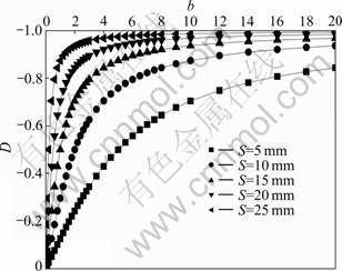
Fig.9 Relationship between D and b with different movements

4.3 Example 2

The numerical analysis of the magnitude and distribution of passive and active earth pressure against rigid retaining wall were preformed by CHEN et al [17-18]. The wall was modeled as a plane-strain, two-dimensional problem for the finite element analysis. As shown in Fig.10, the numerical model was 3 000 mm- wide, 1 200 mm-high and the height of the rigid wall was 1 000 mm. One eight-node quadrilateral element was used to model the soil and one six-node interface element based on the Goodman was employed to model the interaction between the soil and wall. In total, there were 240 elements in the soil mesh and 10 elements in the interface mesh, respectively. The soil elements were modeled as Mohr-Coulomb material and associated flow conditions were assumed. The nodal points at the bottom boundary were fixed, and those on the side boundaries were fixed only in the horizontal direction. The disturbance parameters of backfill are listed in Table 2.

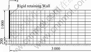
Fig.10 Finite element discretization of experiment model (Unit: mm) [17]

4.3.1 Active condition

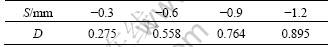
Put the values of S, S_a, S_p and b into Eq.(2), the disturbed degree for each case can be calculated, as listed in Table 3.

Table 2 Material parameters of backfill

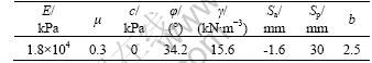
Table 3 Disturbed degree of backfill in active condition

By utilizing the calculated value of D (Table 3) and Eq.(8) and Eq.(9), the lateral earth pressures predicted at different depths are shown in Fig.11. The variation of lateral earth pressures simulated by FEM under different disturbed degrees is also shown in Fig.11.

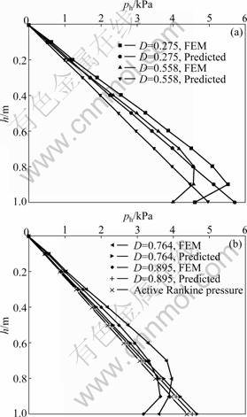
Fig.11 Distributions of active earth pressure under different disturbed degrees

As illustrated in Fig.11, the predicted horizontal earth pressures corresponded closely to the results of FEM around the top of the wall. However, around the bottom of the wall, the horizontal earth pressures of FEM abruptly decreased due to the boundary effect. However, the predicted results increased linearly along the depth of the wall which was more close to the actual distribution of earth pressures. Furthermore, the time on establishing the FEM model was saved. Therefore, the proposed method has higher computational efficiency than FEM.

The variation of horizontal earth-pressure coefficient (K_a) in active condition against disturbed degree (D) is shown in Fig.12. Herein, the coefficient of the predicted earth pressures is denoted by the symbol  and the coefficient of the simulated earth pressures by FEM is denoted by the symbol  The symbol K_a denotes the active coefficient of earth pressure. From Fig.12, it can be seen that  and  decrease non-linearly with the increase of disturbed degree and little difference is observed between them with the same value of D. As D approaches to 1,  and  approach to K_a. Then, the backfill reaches active Rankine state.

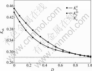
Fig.12 Curves of coefficient of active earth pressure versus disturbed degree

4.3.2 Passive condition

Put the values of S, S_a, S_p and b into Eq.(2), the disturbed degree for each case can be calculated, as shown in Table 1. By utilizing the calculated value of D (Table 1) and Eq.(8) and Eq.(9), the lateral earth pressures predicted at different depths are shown in Fig.13. The variations of lateral earth pressure simulated by FEM under different disturbed degrees are also shown in Fig.13.

As illustrated in Fig.13, the lateral earth pressure increases whereas the disturbed degree decreases. When D approaches to -1, the backfill reaches passive Rankine state. Then, the predicted distribution of earth pressure coincides with that of passive Rankine state. The difference between the simulated earth pressures by FEM and predicted results is little. Moreover, the distribution of the predicted earth pressure agrees well with that of FEM.

The variation of horizontal earth-pressure coefficient (K_p) in passive condition against disturbed degree (D) is shown in Fig.14. Herein, the coefficient of the predicted earth pressures is denoted by the symbol  and the coefficient of the simulated earth pressures by FEM is denoted by the symbol  The symbol K_p denotes the passive coefficient of earth pressure. From Fig.14, it can be seen that  and  increase non-linearly with the decrease of disturbed degree and little difference is observed between them. As D approaches to 1,  and  approach to K_p. Then, the backfill reaches passive Rankine state.

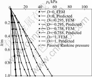
Fig.13 Distributions of passive earth pressure under different disturbed degrees

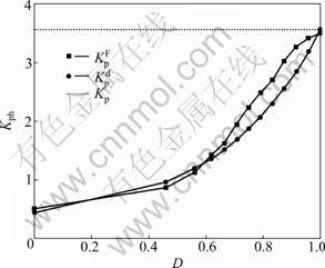
Fig.14 Curves of coefficient of passive earth pressure versus disturbed degree

5 Conclusions

Based on the disturbed state concept (DSC) theory, a general disturbance function for cohesionless backfill was presented. In this function, the at-rest state for backfill was taken as the RI state and both the active and passive Rankine states were considered to be the FA state. The parameters for the function could be obtained from the measured wall movements in translation mode. A novel approach that was related to disturbed degree and the mobilized internal frictional angle of the backfill was also derived. Benefited from Rankine’s theory, the calculation method to predict the actual magnitude and distribution of lateral earth pressure was established. Compared with the test data and predicted results of FEM, it is found that the proposed method can predict the magnitudes and distributions of earth pressures quite well. Furthermore, the proposed method has higher computational efficiency than FEM. The discussion on the influence of the parameter b on the disturbed degree is also presented. It is shown that the rational value of b ranges from 0.5 to 5.

On the other hand, it should be pointed out that the proposed method is highly simplified. It does not cover many complex conditions of the wall movement modes such as rotation about a point above the top (RTT mode) and below the wall base (RBT mode). The application of disturbed theory to the above two movement modes will be further studied.

References

[1] FANG Y S, ISHIBASHI I. Static earth pressures with various wall movements [J]. Journal of Geotechnical and Geoenvironmental Engineering, ASCE, 1986, 112(3): 317-333.

[2] DUNCAN J M, WILLIAMS G W, SEHN A L, SEED R B. Estimation earth pressures due to compaction [J]. Journal of Geotechnical and Geoenvironmental Engineering, ASCE, 1991, 117(2): 1833-1847.

[3] FANG Y S, CHEN J M, CHEN C Y. Earth pressures with sloping backfill [J]. Journal of Geotechnical and Geoenvironmental Engineering, ASCE, 1997, 123(3): 250-259.

[4] FANG Y S, HO Y C, CHEN T J. Passive earth pressure with critical state concept [J]. Journal of Geotechnical and Geoenvironmental Engineering, ASCE, 2002, 128(8), 651-659.

[5] CLOUGH G W, DUNCAN J M. Finite element analyses of retaining wall behaviour [J]. Journal of the Soil Mechanics and Foundation, ASCE, 1971, 97(12): 1657-1673.

[6] NAKAI T. Finite element computations for active and passive earth pressure problems on retaining wall [J]. Soil and Foundation, 1985, 25(3): 98-112.

[7] XU R Q, CHEN Y K, YANG Z X, GONG X N. Experimental research on the passive earth pressure acting on a rigid wall [J]. Chinese Journal of Geotechnical Engineering, 2002, 24(5): 569-575. (in Chinese)

[8] DESAI C S. A consistent finite element technique for work softening behavior [C]// Proc Int Conf on Computer Methods in Nonlinear Mechanics. Austin: University of Texas, 1974: 969-978.

[9] KATTI D R, DESAI C S. Modeling and testing of cohesive soil using disturbed state concept [J]. Journal of Engineering and Mechanics, ASCE, 1995, 121(5): 648-658.

[10] DESAI C S, WANG Z C. Disturbed state model for porous saturated materials [J]. International Journal Geomechanics, ASCE, 2003, 3(2): 260-264.

[11] EI-HOSEINY K E, DESAI C S. Prediction of field behaviour of reinforced soil wall using advanced constitutive model [J]. Journal of Geotechnical and Geoenvironmental Engineering, ASCE, 2005, 131(6): 729-739.

[12] PRADHAN S K, DESAI C S. DSC model for soil and interface including liquefaction and prediction of centrifuge test [J]. Journal of Geotechnical and Geoenvironmental Engineering, ASCE, 2006, 132(2): 214-222.

[13] WILLIAM L T, WHITMAN R V. Soil mechanics [M]. SI Version. New York: John Wiley & Sons, 1979: 123-126.

[14] PARK I J, DESAI C S. Cyclic behavior and liquefaction of sand using disturbed state concept [J]. Journal of Geotechnical and Geoenvironmental Engineering, 2000, 126(9): 834-846.

[15] DESAI C S. Mechanics of materials and interfaces: The disturbed state concept [M]. Boca Raton, CRC Press, 2001: 875-883.

[16] MEI Guo-xiong, ZAI Jin-min. Rankine earth pressure model considering deformation [J]. Chinese Journal of Rock Mechanics and Engineering, 2001, 20(6): 851-853. (in Chinese)

[17] CHEN Ye-kai, WANG Yi-min, XU Ri-qing, GONG Xiao-nan. Numerical analysis of passive earth pressure on rigid retaining wall [J]. Chinese Journal of Rock Mechanics and Engineering, 2004, 23(6): 980-988. (in Chinese)

[18] CHEN Ye-kai, WANG Yi-min, XU Ri-qing, GONG Xiao-nan. Numerical analysis of active earth pressure on rigid retaining wall [J]. Chinese Journal of Rock Mechanics and Engineering, 2004, 23(6): 989-995. (in Chinese)

(Edited by YANG Bing)

Foundation item: Project(50678158) supported by the National Natural Science Foundation of China

Received date: 2010-07-04; Accepted date: 2010-12-30

Corresponding author: XU Ri-qing, Professor, PhD; Tel: +86-571-88206398; E-mail: xurq@zju.edu.cn