J. Cent. South Univ. (2020) 27: 2711-2725

DOI: https://doi.org/10.1007/s11771-020-4493-9

Locating microseismic sources based upon L-shaped single-component geophone array: A synthetic study

DING Liang(丁亮)^{1, 2}, LIU Qin-ya(刘沁雅)^{2, 3}, GAO Er-gen(高尔根)⁴,QIAN Wei(钱卫)¹, SUN Shou-cai(孙守才)⁵

1. School of Earth Sciences and Engineering, Hohai University, Nanjing 211100, China;

2. Department of Physics, University of Toronto, Toronto ON M5S 1A7, Canada;

3. Department of Earth Sciences, University of Toronto, Toronto ON M5S 3B1, Canada;

4. School of Civil Engineering, Anhui Jianzhu University, Hefei, China;

5. School of Earth Sciences, Institute of Disaster Prevention, Beijing 101601 China

Central South University Press and Springer-Verlag GmbH Germany, part of Springer Nature 2020

Abstract: We have developed a type of L-shaped single-component geophone array as a single station (L-array station) for surface microseismic monitoring. The L-array station consists of two orthogonal sensor arrays, each being a linear array of single-component sensors. L-array stations can be used to accurately estimate the polarization of first arrivals without amplitude picking. In a synthetic example, we first use segmentally iterative ray tracing (SIRT) method and forward model to calculate the travel time and polarization of first arrivals at a set of L-array stations. Then, for each L-array station, the relative delay times of first arrivals along sensor arrays are used to estimate the polarization vector. The small errors in estimated polarization vectors show the reliability and robustness of polarization estimation based on L-array stations. We then use reverse-time ray-tracing (RTRT) method to locate the source position based on estimated polarizations at a set of L-array stations. Very small errors in inverted source location and origin time indicate the great potential of L-array stations for source localization applications in surface microseismic monitoring.

Key words: geophone array; polarization; source location; seismic monitoring

Cite this article as: DING Liang, LIU Qin-ya, GAO Er-gen, QIAN Wei, SUN Shou-cai. Locating microseismic sources based upon L-shaped single-component geophone array: A synthetic study [J]. Journal of Central South University, 2020, 27(9): 2711-2725. DOI: https://doi.org/10.1007/s11771-020-4493-9.

1 Introduction

Polarization is an important attribute of seismic wave, for it provides the propagating direction of seismic wave and can be used in real-time source position determination [1-6]. Polarization can be estimated by using the amplitude of multi-component seismic data recorded by single station or station array on free surface, which is called the particle motion direction [7-10]. PARK et al [11] pointed out that as the first-arrival particle motion recorded on free surface is the superposition of incident P waves, the reflected P waves and reflected SV waves, the polarization direction of the incident waves is not the same as the surface particle motion direction (also known as apparent polarization direction), and needs to be converted based on near-surface structures [7, 10]. The incident direction of seismic wave can be calculated by using the accurate nearsurface velocity structure and the particle motion direction which is obtained from three-component (3-C) seismic data recorded by single station and station array on surface.

The 3-C recordings from single station can be used to estimate the apparent polarization [2, 4, 8, 9, 12-14]. The amplitude of seismic waveform is used for the estimation. For example, VIDALE [8] projected 3-C seismic recordings onto three orthogonal axes to form a covariance matrix, and the eigenvector associated with the largest eigenvalue is regarded as the direction of the largest amount of polarization. The eigendecomposition of covariance matrix for polarization estimating is well developed [2, 15]. MAGOTRA et al [1] used the amplitudes of horizontal components to estimate the azimuth of incident P wave, and the polarization is used to locate the source position. GALIANA-MERINO et al [13] used an adaptive- length window to construct a covariance matrix and calculates the eigenvector associated with the maximum eigenvalue to determine the azimuth of P wave. DING et al [4] used a sliding window to scan the 3-C time series in the range which contains the first break and determine the particle motion direction by the spread of vector in sliding window without calculating the eigenvalues and eigenvectors. Other method such as the principle component analysis (PCA) projects 3-C seismic recordings onto the vertical radial plane to build the covariance matrix, and the eigenvector associate with the maximum eigenvalue is regarded as the principle direction of polarization [11]. Those estimation methods depend on the precise phase detection and amplitude picking. The errors in phase detection and phase picking cause wrong polarization, and the reliability of amplitude picking is reduced because of the inaccuracy of near-surface velocity structures, low SNR and unknown source types.

Polarization can be estimated based on seismic array data, and the estimating methods are well developed [9, 16-20]. ROST et al [9] pointed out that the array methods to estimate the polarization assume the seismic waves arriving at the array to be plane waves. Station array takes advantages of the different spatial correlation properties of seismic signals, noise and local scattering effects and enhance signal quality in certain frequency bands [21]. Under the plane wave assumption, the seismic signals from different stations in array are correlated while the random noise and local scattering effects are not. Therefore, measuring the amplitude of plane wave at stations or knowing the arrival time of plane wave at station array allows a direct measure of the polarization. Amplitude of seismic wave recorded by station array can be used for polarization estimating. For example, JURKEVICS [21] computed the polarization by solving the eigen problem of the covariance matrix within sliding time window for individual sensor and reduces the estimation variance of polarization attributes by averaging covariance matrices for the different sensors. LA ROCCA et al [18] stacked the seismograms recorded at array stations to improves the SNR directly without time shift because of the small array length and high apparent velocity. The stacked seismograms are used to estimate the polarization of low-frequent events. BAYER et al [2] tracked the rapture procedure of huge earthquake using the changes of P polarization estimated from 3-C seismic recordings at 5 stations. These estimating methods dependent on amplitude picking are disturbed by noise. The background noise reduces the reliability of phase detecting and amplitude picking, which results in a random polarization. The estimating result based on surface recordings is particle motion direction, which is called apparent polarization, caused by incident and reflected P wave and reflected SV wave rather than the direction of incident P vector. The apparent polarization needs to be corrected by accurate velocity structure to get the incident polarization.

Other estimating methods are based on travel time of seismic recordings from station array [9, 16, 22, 23]. With the plane wave assumption, the arrival time of seismic wave is dependent on the source and station position, velocity structure which can be obtained by geophysical survey, and incident angle. In turn, knowing the station positions and the travel time difference of seismic wave at the station array therefore allow a direct estimation of the polarization. For example, DAVIES et al [16] used time delays of the seismic signal recorded at the station array and provided a direct estimating method for calculating the back azimuth and the slowness, which was called velocity spectral analysis (Vespa) process. ROST et al [9] used the differential travel times of the plane wave front observed in array stations to estimate the azimuth of seismic wave. FOSTER et al [22] used arrival time difference to find the source position with the minimum misfit of travel time difference and then determined the arrival angle and the back azimuth. These methods take advantages of the arrival time rather than the amplitude of seismic signal to estimate the polarization because they avoid the disturbance of the inaccuracy of amplitude picking and do not need to correct the apparent polarization to get incident direction.

Large station array coincides with the research of low frequency seismic waves generated by the source such as teleseismic and tremor because of the assumption that the seismic wave fronts recorded at the station array are regarded as plane wave [2, 18, 21, 24, 25]. Small station arrays, such as star-shaped array [26-28], large-N array [29, 30] and the patch array [23, 31] are deployed for observing the seismic wave generated by microseismic events that are induced during the hydraulic fracturing process. Other geophone arrays made up of several sensors are commonly used as individual station in seismic exploration, and the amplitude stacking of recording of each sensor within a station can improve the SNR [32, 33]. The individual station which consisted with several single component sensors, such as the vertical sensor, can record the arrival time of seismic wave passing through the sensor array, and the travel time difference of seismic wave can be used for estimating the polarization. The estimating method is dependent on the arrival time of seismic wave rather than the amplitude and is insensitive to the inaccuracy of amplitude picking.

In this research, we propose to use an L-shaped orthogonal single-component geophone array as a single station (we call an L-array station) to estimate the polarization of the first break. Once polarizations of the first break at different stations are determined, the source location can be accurately inverted by reverse time ray-tracing method (RTRTM) [4]. In the following sections, we first present a brief theoretical introduction to the L-array station and the polarizations analysis method, and then demonstrate the use of L-array stations for microseismic source location determination by a synthetic example.

2 L-array station

Large aperture arrays consisting of seismic stations with large inter-site spacing have commonly applied for earthquake monitoring [34]. For example, HICKS et al [35] used two local temporary networks to estimate the epicenter of a set of low-magnitude earthquakes. LI et al [36] used a small-aperture temporary seismic array and the arrival times of P and S-P to locate the source position. LI et al [37] used the US seismic network as a large aperture array to image the rupture process of the 2015 M_w8.3 Illapel earthquake.

Large aperture arrays with specific shape can be utilized to estimate the attributes of seismic wave. Such as the L-shaped array, formed by two perpendicular surface sensor arrays, has been used to measure the rotational component of teleseismic surface waves [38], and solve the directions-of- arrival (DOA) estimation problems [39-41]. For example, large L-shaped array with several kilometer spacing for the Interferometer Gravitational-Wave Observatory (LIGO) Hanford Observatory (LHO) has been used to measure the horizontal rotational motion of Rayleigh waves from teleseismic events [38], and the L-shaped broadband seismic array situated on the Jurassic limestone of the Franconian Alb in SE Germany, known as the GRF array, has been used to detect the earthquake [9, 42].

The L-array station that we proposed for polarization estimation is an L-shaped surface array formed by two perpendicular geophone arrays, each with a line of single component sensors arranged along the left array or the right array, as shown in Figure 1. These sensors in the left (or right) array (inverted triangles in Figure 1) are marked as L (or R) with increasing numbers as sensors move away from the sensor (denoted as L_R) at the intersection point of the left and right array. In practice, sensor spacing, and the number of sensors in each array can be configured based on the terrain setting and geophysical purposes. The L-array station shown in Figure 1 has five sensors with even spacing of 1.0 m in each array. The right array is usually aligned in the east direction (i.e., x axis), the left array is along the north direction (i.e., y axis), and the vertical upward direction is regarded as the z axis.

Figure 1 A single L-array station consisting of two orthogonal single-component geophone arrays (the left array and right array) (Geophones (black inverted triangles) are deployed with spacing of 1.0 m along two orthogonal lines (dash lines))

3 Polarization estimation method

If we assume that the array aperture of an L-array is much smaller than the distance between sources and the station, then the arriving body waves at the station from distant microseismic source can be treated as plane waves in the near surface.

Polarization estimation can take advantage of this plane wave approximation. As the wavefronts approach the surface (Figure 2), the relative delay of arrival time at each sensor is closely related to the incident angle of incoming waves, azimuth of surface array, and sensor spacing. For example, compared to the L_R sensor, the relative arrival time delay for the other sensors in the right array can be calculated by:

               (1)

where △t_i is the arrival time delay of the i-th sensor compared to the L_R sensor △t₁=0; r_j is the right array spacing between the j-th and (j+1)-th sensor; φ is the azimuth of surface projection of the ray vector; V is the velocity of near-surface layer. By assuming that apparent velocity of the arrival waves does not change along the array, the apparent velocity along the right array is given by:

           (2)

Figure 2 (a) Plane waves arriving at the surface with an incident angle of θ is shown in the vertical cross-section perpendicular to the wavefronts. Seismic rays are shown in dashed lines and the corresponding wave fronts are shown as thick lack lines. The surface spacings between wavefronts are denoted by d_i. The velocity of near-surface medium is V; (b) A map view of left and right array sensor array and surface intersections of wavefronts (dashed lines) shown in (a). The array spacings for the left array and right array are l_i and r_i. The propagation velocity of wavefronts along the surface is the apparent velocity, which is denoted as V⁰. V_R and V_L are the apparent velocity of wavefronts observed along right and left array

The near surface medium velocity V can be estimated based on other geophysical survey data, such as well-log recordings or reflection seismic. Similarly, the relative delay times between the left array sensors are given by:

               (3)

And the apparent velocity along the left array becomes:

           (4)

Once the right apparent velocity (Eq. (2)) and left apparent velocity (Eq. (4)) are obtained, the polarization vector P of the plane waves arriving at an L-Array station can be calculated by:

        (5)

There are three special cases to be considered. If the plane waves propagate along the right array, i.e., the azimuth of the surface projection of ray vectors is 0 (φ=0), then the waves arrive at the same time on the left array sensors, which makes the left apparent velocity (V_L) infinity theoretically, and we can rewrite this polarization vector as:

                   (6)

Similarly, if the plane waves propagate along the left array and perpendicular to the right array (φ=90°), then the right apparent velocity (V_R) becomes infinite, and we can rewrite the polarization of arrival as:

                   (7)

If the seismic ray arrives vertically beneath the L-array and the wavefronts are parallel to the surface plane determined by L-array station, the relative arrival delays on both the left and right array sensors are zero, which makes both the left and right apparent velocity infinite. In this case, the polarization of arrival waves becomes:

P=(0, 0, 1)                              (8)

In general, once the right apparent velocity (V_R) and the left apparent velocity (V_L) are determined, the average polarization direction for this L-array station can be estimated based on Eq. (5). To accurately determine the left and right apparent velocity, we use a velocity scanning method to select the optimal velocity corresponding to the highest stacked amplitude, as discussed in detail in Section 4.2.

4 Synthetic example

In this section, using a synthetic example, we show how arrival polarization and source location can be determined based on a set of L-array stations. We first perform a forward modeling for a known velocity model to construct synthetic waveforms arrival at a set of L-array stations. We then apply velocity scanning methods to calculate the velocity spectrum [33] and select the velocity corresponding to the maximum amplitude of velocity spectrum as the directional apparent velocities for the left and right array, which are then used for calculating polarization directions at each L-array station. These polarization vectors are further used to estimate the seismic source location based on reverse-time ray-tracing (RTRTM) techniques [4]. This methodology is applicable to both P and S arrivals, and we will use the first P arrivals as an example in the modeling below.

4.1 Forward modeling

To obtain synthetic waveforms for arrivals at a set of test L-array stations, we first define a complex three-dimensional layered background model with six undulating velocity interfaces. The velocity for each layer between two neighboring interfaces is constant as given by Table 1. The top interface with the elevation of 500.0 m is horizontal and regarded as the surface. The second interface is also horizontal with an altitude of 100.0 m. The next four interfaces are defined by undulating sinusoidal functions with average depths at -500.0, -1000.0, -1500.0, -2000.0 m, respectively.

Table 1 Velocity model used for forward ray tracing and source inversion (z=0 indicates the sea)

We then place a source (star in Figure 3) at position (-1000.0, -1000.0, -2500.0) m, and five L-array stations (numbered L-shaped signs in Figure 3(a)) with their L_R sensors at (1000.0, 1000.0, 500.0) m, (1000.0, 500.0, 500.0) m,(1000.0, 0, 500.0) m, (1000.0, -500.0, 500.0) m, (1000.0, -1000.0, 500.0) m (Figure 3). The left and right sensor arrays of an L-array station contain 5 sensors each with a spacing of 1.0 m. The left array is aligned with the Y axis, while the right array is along the X axis. A vertical cross-section view (Figure 3(b)) shows the layout of L-array stations and source in depth. We assume that the initial time of event is 00 : 00 : 00.

Figure 3 Map view (a) and depth view (b) of microseismic source and L-array stations geometry (The five L-array stations are deployed on the surface with their L_R sensors at (1000.0, 1000.0, 500.0) m, (1000.0, 500.0, 500.0) m, (1000.0, 0, 500.0) m)

We use the segmentally iterative ray tracing (SIRT) method [43-48] to calculate the travel time and polarity vector of first break at each sensor of an L-array station for the 3D background model. SIRT is a ray bending method that achieves two-point ray tracing by adjusting the intersection points of seismic rays and interfaces iteratively. We use a Ricker wavelet as the source wavelet given by the formula:

                       (9)

where a=0.02 ms is the half duration of the central peak, setting the zero time to be at the peak of the Ricker wavelet. We then place the peak of the wavelet at the predicted arrival times from SIRT to generate waveforms for the first-break at various sensors (Figure 4). The sampling rate of the waveforms is 1 MHz, and we generate up to 2 ms of data. Five single-component waveforms from the left and right array are shown in Figure 4.

4.2 Velocity scanning

We use velocity scanning method to estimate the most likely directional apparent velocities along the left array and right array. We create an image of stacked amplitude as a function of time and velocity, and then select the velocity corresponding to the maximum amplitude as the directional apparent velocity. Specifically, we regard the L_R sensor (sensor with index 1 in Figure 4) as the base sensor, and the waveform for the L_R sensor as the base trace, and select an appropriate scanning time window from on L_R trace (dash rectangle on L_R trace in Figure 4), and a series of scanning velocities. For a selected time in the scanning time window and a selected velocity, we calculate the predicted arrival time delay (e.g., dashed lines in Figure 4) of the first-break as a function of distance from the L_R sensor. We can then select the amplitude of the waveform at each sensor corresponding to the time in the relative delay curve and stack these amplitudes. Figure 5 shows the variation of stacked amplitude as a function of time and velocity for the left and right arrays of the five L-array stations. If the scanning time corresponds to the peak of seismic phase (in this example the peak of the Ricker wavelet in L_R trace), and the scanning velocity is close to the real directional apparent velocity, the times selected by the relative delay curve will have large amplitudes and stack coherently to give a peak in the amplitude image.

We perform velocity scanning on the synthetic first-break waveforms and obtain the stacked amplitude images of the left and right arrays (Figure 5) for L-array station 1-5. In this example, scanning time window length is 0.25 ms, and the scanning velocities range from 3000 to 6000 m/s for the right array with an increment of 10 m/s, while the velocity ranges for the left array varies for different stations (see Figure 5 for details). The highest stacked amplitude is identified by ‘+’ on Figure 5 and is considered to correspond to the directional apparent velocity for the array, and the arrival time at the L_R sensor (which is the same for the left and right array). At L-array station 1, the left apparent velocity is 4730 m/s (Figure 5(a)), which is equal to the right apparent velocity (Figure 5(b)). At L-array station 2, the left apparent velocity is 5910 m/s (Figure 5(c)) which is higher than the right apparent velocity of 4440 m/s (Figure 5(d)). At L-array station 3, the left apparent velocity is 8410 m/s (Figure 5(e)) while the right apparent velocity is 4210 m/s (Figure 5(f)). At L-array station 4, the left apparent velocity is 16100 m/s (Figure 5(g)), significantly higher than the right apparent velocity of 4080 m/s (Figure 5(h)). At L-array station 5, the left apparent velocity is huge (Figure 5(i)), and the right apparent velocity is 4020 m/s (Figure 5(j)). From the analysis of special cases in section 3, in combination with the source receiver geometry in Figure 3, this is clearly a result of the alignment of right array in the direction of wave propagation from the source for L-array station 5. Assuming relatively small variations in incident angle across stations, the increase in V_L and decrease in V_R from station 1 to 5 reflect the fact that source-receiver paths become more aligned with the right array from station 1 to 5.

Figure 4 Synthetic waveforms along (left panels) (a, c, e, g, i) and (right panels) (b, d, f, h, j) for array sensors at five L-array stations (station 1 at top to station 5 at bottom) (Velocity scanning (dashed lines) is performed for a range of scanning time and velocities for amplitude stacking)

Figure 5 Stacked amplitude images from velocity scanning for L-array station 1 to 5 (top to bottom) (The maximum amplitude is indicated by ‘+’ in each plot, and the corresponding velocity is considered to be the apparent velocity along the array while the corresponding time gives the arrival time of the L_R sensor)

4.3 Polarization estimation and source location

With the estimated apparent velocities along left and right arrays of the L-array stations, we can calculate the polarization of first break based on Eq. (5). The original and inverted surface, left-array, right-array apparent velocities, and the polarization vector (represented as azimuth and incident angle) are listed in Table 2. The relative errors between the forward and inverted result are generally quite small (less than 0.5%), which shows the validity of the plane-wave incidence assumption and reliability of velocity scanning method in estimating the polarization direction. Furthermore, we use the inverted polarization vectors and arrival time of first break at L_R traces for these five L-array stations to locate the seismic source based on the reverse- time ray-tracing methods [4]. With the same background velocity model as the one used in the forward modeling (Table 1), we use the arrival times determined from the velocity scanning analysis, and trace back the seismic rays from the L_R sensors at five L-array stations with the estimated polarization vectors as the initial ray vectors. Ideally, these back-traced seismic rays should converge back to the original source position at the initial time. We back-trace the seismic rays from five L_R sensors at each L-array station time-reverse and use the average distant between terminals and their central point to monitoring whether terminals converge. The terminal points converge to the source at 00: 00: 00, which equals the initial time that we set at Section 4.1. Figure 6 shows the changing of the position errors for x, y and z components (estimated from the closeness of ray terminals) with the time when ray terminals are close to the converging source position. The position errors for x, y and z components all decrease with the time close to the initial time 00: 00: 00, as all ray terminals gradually focus. It represents the seismic rays travel time-reverse and approach to the source. However, before 00: 00: 00, the time before event, the ray terminals separate out again, with gradually increasing position errors. The ray terminals within this time represent nothing but mathematical meanings. Clearly all seismic rays converge at 00: 00: 00 which is also the initial time of event that we assumed in Section 4.1.

Table 2 Result of forward and inverted apparent velocity and polarization

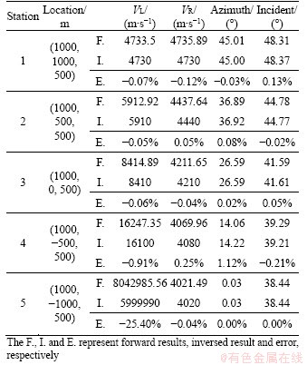
Figure 6 Error bars of x (a), y (b), z (c) component of source position as a function of time estimated from closeness of ray terminals

We also obtain that the final inverted source position is at (-1000.47, -1000.20, -2500.40) m, while the original source position is at (-1000, -1000, -2500) m, and the corresponding source position error is about 0.05%, 0.02% and 0.02% in the x, y and z directions. These small errors show the robustness in microseismic source location estimation by RTRTM and L-Array stations.

5 Discussion

Near-surface structures strictly influence the propagation direction of seismic wave. The incorrect velocity structure causes the polarization estimation based on the amplitude of seismic recordings inaccurate. For instance, the estimation of incident P ray direction requires correction to get the real direction by combining the particle motion direction with near-surface SV structure [11]. DING et al [4] used 3-C seismic recordings to estimate the particle motion direction and correct the incident P ray direction by combining the near-surface SV structure and point out that the inaccuracy of surface SV structure reduces the reliability in source depth.

The polarization estimation by L-array stations relies on surface P structure. Using the forward results (Table 2), we calculate the incident direction in three surface structures with different P wave velocity which are 2000, 2500, 3000 m/s. The results obtained for 2500 m/s are equivalent to the inversed results listed in Table 2.

Polarization estimating methods based on the amplitude of seismic recordings from single station or station array face the challenges of the low SNR, the inaccuracy of near-surface structures and unknown source type. Even surface geophone arrays have been proposed to strengthen the SNR [23, 26], the noise could reduce the reliability of amplitude picking and cause random polarization. Despite the influence of noise, the polarization of first break estimated from surface recordings is the particle motion direction, which is the superposition of incident and reflected P wave and reflected SV wave [7, 10]. To get the incident direction, the particle motion direction should be corrected by using accurate near-surface structure. Those methods based on the amplitude of seismic recordings to estimate the polarization require the precision of phase detection and amplitude picking. Those are sensitive to the inaccuracy of amplitude picking.

Other methods use travel time of first break recorded by station array to estimate the polarization of first break. Those methods take advantage of plane wave assumption and can be used to estimate the azimuth of first break without picking the amplitude value from seismic recordings [9]. We propose a polarization estimation approach based on travel time and L-array stations, a geophone layout with two orthogonal single-component sensor arrays. These arrays are less costly and logistically easier to deploy than three-component sensors for a single station [13], and do not require amplitude picking for polarization estimation. The polarization estimation based on L-array stations does assume plane-wave incidence. In this paper, we choose the sensor spacing in the left and right array as 1.0 m to detect a plane-wave incidence with a Ricker wavelet of ~0.1 ms length, sampled at a rate of 1 MHz by geophones. In practice, for sensors in an L-array station to record different arrival delay of the same phase, sensor spacing should be at least several times bigger than the product of the directional apparent velocity and sampling rate.

Figure 7 Noise added to waveform (The meanings of the vertical and horizontal axes is the same as Figure 4)

Compared to a low-sampling-rate data, a high- sampling-rate record can provide higher temporal resolution for arrival delay measurements under the same sensor spacing and directional apparent velocity. On the other hand, stretching the sensor spacing too much or adding more sensors in an array will increase the aperture of the array, and therefore make the plane-wave incidence assumption less accurate. It will also increase the error on apparent velocity measurements as the polarization at the L_R sensor may not be a good approximation of the average polarization for all sensors at L-array station. Therefore, sensor spacing and the number of sensors need to be adjusted based on the intended geophysical applications. The L-array stations can be used for accurate microseismic source localization without polarization correction as required by conventional 3C surface microseismic monitoring array [49].

Figure 8 Amplitude stacking performed using waveforms containing noise (The meaning of the vertical and horizontal axes is the same as Figure 5)

Figure 9 Error bars of x (a), y (b), z (c) component of source position as a function of time (The source location is obtained by using the wave form containing noise)

Table 3 Incident direction estimated from different surface velocity structure

6 Conclusions

We conceptually propose an L-array station with two orthogonal single-component sensor arrays for the purpose of robust polarization estimation at the station. The apparent velocity along the left or right array can be extracted based on a velocity scanning method. The polarization vector of the first break (e.g., incidence angle and azimuth) can then be calculated from the left and right apparent velocity, as well as the velocity at near-surface. As shown by our synthetic example, through automatic velocity scanning, the recovered polarization directions coincide well with those from the forward modeling. These polarization vectors at various L-array stations can be further used to determine the source position based on the reverse-time ray-tracing method. In our synthetic example, the final inverted source position is also close to the original source position with very small relative errors. The well-recovered results in the synthetic example show the reliability of the polarization estimation and source localization based on L-array stations. L-array stations using high sampling-rate single-component geophone sensors are cost-effective and easy to deploy in practice. Therefore, we foresee great potential for the application of L-array stations in surface microseismic monitoring.

Contributors

DING Liang conducted the study and edited the draft of manuscript. LIU Qin-ya helped to revise the draft of manuscript. GAO Er-gen provided suggestions on source localization. SUN Shou-cai presented the idea of the velocity scanning. QIAN Wei helped to conduct the numerical test.

Conflict of interest

DING Liang, LIU Qin-ya, GAO Er-gen, QIAN Wei and SUN Shou-cai declare that they have no conflict of interest.

References

[1] MAGOTRA N, AHMED N, CHAEL E. Single-station seismic event detection and location [J]. IEEE Transactions on Geoscience and Remote Sensing, 1989, 27(1): 15-23. DOI: 10.1109/36.20270.

[2] BAYER B, KIND R, HOFFMANN M, YUAN X, MEIER T. Tracking unilateral earthquake rupture by P-wave polarization analysis [J]. Geophysical Journal International, 2012, 188(3): 1141-1153. DOI: 10.1111/j.1365-246X.2011. 05304.x.

[3] HIRABAYASHI N. Real-time event location using model-based estimation of arrival times and back azimuths of seismic phases [J]. Geophysics, 2016, 81(2): KS25-KS40. DOI: 10.1190/geo2014-0357.1.

[4] DING Liang, GAO Er-gen, LIU Qin-ya, QIAN Wei, LIU Dong-dong, YANG Chi. Reverse-time ray-tracing method for microseismic source localization [J]. Geophysical Journal International, 2018, 214(3): 2053-2072. DOI: 10.1093/GJI/ GGY256.

[5] PARK S, ISHII M. Detection of instrument gain problems based on body-wave polarization: Application to the Hi-Net array [J]. Seismological Research Letters, 2019, 90(2A): 692-698. DOI: 10.1785/0220180252.

[6] PARK S, TSAI V C, ISHII M. Frequency-dependent p wave polarization and its subwavelength near-surface depth sensitivity [J]. Geophysical Research Letters, 2019, 46(24): 14377-14384. DOI: 10.1029/2019GL084892.

[7] XU Guo-ming, ZHOU Hui-lan. Priciples of seismology [M]. Beijing: Science Press, 1982. (in Chinese)

[8] VIDALE J E. Complex polarization analysis of particle motion [J]. Bulletin of the Seismological Society of America, 1986, 76(5): 1393-1405.

[9] ROST S, THOMAS C. Array seismology: Methods and applications [J]. Reviews of Geophysics, 2002, 40(3): 1008. DOI: 10.1029/2000RG000100.

[10] SHEARER P M. Introduction to seismology [M]. 2nd Ed. Cambridge: Cambridge University Press, 2009, DOI: 10.1016/B978-0-444-56375-0.00020-7.

[11] PARK S, ISHII M. Near-surface compressional and shear wave speeds constrained by body-wave polarisation analysis [J]. Geophysical Journal International, 2018, 213: 1559-1571. DOI: 10.1093/gji/ggy072.

[12] ANANT K S, DOWLA F U. Wavelet transform methods for phase identification in three-component seismograms [J]. Bulletin of the Seismological Society of America, 1997, 87(6): 1598-1612.

[13] GALIANA-MERINO J J, ROSA-HERRANZ J, JAREGUI P, MOLINA S, GINER J. Wavelet transform methods for azimuth estimation in local three-component seismograms [J]. Bulletin of the Seismological Society of America, 2007, 97(3): 793-803. DOI: 10.1785/0120050225.

[14] OHTA K, ITO Y, HINO R, OHYANAGI S, MATSUZAWA T, SHIOBARA H, SHINOHARA M. Tremor and inferred slow slip associated with afterslip of the 2011 Tohoku earthquake [J]. Geophysical Research Letters, 2019, 46(9): 4591-4598. DOI: 10.1029/2019GL082468.

[15] D’AURIA L, GIUDICEPIETRO F, MARTINI M, ORAZI M, PELUSO R, SCARPATO G. Polarization analysis in the discrete wavelet domain: An application to volcano seismology [J]. Bulletin of the Seismological Society of America, 2010, 100(2): 670-683. DOI: 10.1785/ 0120090166.

[16] DAVIES D, KELLY E J, FILSON J R. Vespa process for analysis of seismic signals [J]. Nature Physical Science, 1971, 232(27): 8-13. DOI: 10.1038/physci232008a0.

[17] WAGNER D E, EHLERS J W, VEEZHINATHAN J. First break picking using neural networks [C]// SEG Technical Program Expanded Abstracts 1990. 2005: 370-373. DOI: 10.1190/1.1890201.

[18] LA ROCCA M, GALLUZZO D, MALONE S, MCCAUSLAND W, DEL PEZZO E. Array analysis and precise source location of deep tremor in Cascadia [J]. Journal of Geophysical Research: Solid Earth, 2010, 115(6): B00A20. DOI: 10.1029/2008JB006041.

[19] CRISTIANO L, MEIER T, KRUGER F, KEERS H, WEIDLE C. Teleseismic P-wave polarization analysis at the Grafenberg array [J]. Geophysical Journal International, 2016, 207(3): 1456-1471. DOI: 10.1093/gji/ggw339.

[20] ROSS Z E, MEIER M A, HAUKSSON E. P wave arrival picking and first-motion polarity determination with deep learning [J]. Journal of Geophysical Research: Solid Earth, 2018, 123(6): 5120-5129. DOI: 10.1029/2017JB015251.

[21] JURKEVICS A. Polarization analysis of three-component array data [J]. Bulletin-Seismological Society of America, 1988, 78(5): 1725-1743.

[22] FOSTER A, EKSTROM G, HJORLEIFSDOTTIR V. Arrival-angle anomalies across the USArray transportable array [J]. Earth and Planetary Science Letters, 2014, 402(C): 58-68. DOI: 10.1016/j.epsl.2013. 12.046.

[23] ROUX P F, KOSTADINOVIC J, BARDAINNE T, REBEL E, CHMIEL M, VAN PARYS M, MACAULT R, PIGNOT L. Increasing the accuracy of microseismic monitoring using surface patch arrays and a novel processing approach [J]. First Break, 2014, 32(7): 95-101.

[24] GERSTOFT P, TANIMOTO T. A year of microseisms in southern California [J]. Geophysical Research Letters, 2007, 34(20): 2-7. DOI: 10.1029/2007 GL031091.

[25] ISHII M, SHEARER P M, HOUSTON H, VIDALE J E. Sumatra earthquake ruptures using the Hi-net array [J]. Journal of Geophysical Research: Solid Earth, 2007, 112(11): B11307. DOI: 10.1029/2006JB004700.

[26] CHAMBERS K, KENDALL J M, BRANDSBERG-DAHL S, RUEDA J. Testing the ability of surface arrays to monitor microseismic activity [J]. Geophysical Prospecting, 2010, 58(5): 821-830. DOI: 10.1111/j.1365- 2478.2010.00893.x.

[27] DUNCAN P M, EISNER L. Reservoir characterization using surface microseismic monitoring [J]. Geophysics, 2010, 75(5): 75A139-75A146. DOI: 10.1190/1.3467760.

[28] VLCEK J, FISCHER T, VILHELM J. Back-projection stacking of P- and S-waves to determine location and focal mechanism of microseismic events recorded by a surface array [J]. Geophysical Prospecting, 2016, 64(6): 1428-1440. DOI: 10.1111/1365-2478.12349.

[29] WITTEN B, SHRAGGE J C. Improved microseismic event locations through large-N arrays and wave-equation imaging and inversion [C]// American Geophysical Union, Fall General Assembly 2016. abstract id. S31B-2761., 2016.

[30] LI Ze-feng, PENG Zhi-gang, ZHU Li-jun, MCCLELLAN J. High-resolution microseismic detection and location using Large-N arrays [C]// 2017 Workshop: Microseismic Technologies and Applications. Hefei, 2017: 59-63. DOI: 10.1190/microseismic2017-015.

[31] AUGER E, SCHISSELE-REBEL E, JIA J. Suppressing noise while preserving signal for surface microseismic monitoring: The case for the patch design [G]// SEG Technical Program Expanded Abstracts, 2013: 2024-2028. DOI: 10.1190/ segam2013-1396.1.

[32] SHERIFF R E, GELDART L P. Exploration seismology [M]. Cambridge: Cambridge University Press, 1995. DOI: 10.1017/ CBO9781139168359.

[33] YILMAZ O. Seismic data analysis: Processing, inversion, and interpretation of seismic data [M]. Istanbul, Turkey, 2001. DOI: 10.1190/1.9781560801580.

[34] GIBBONS S J. The applicability of incoherent array processing to IMS seismic arrays [J]. Pure and Applied Geophysics, 2014, 171(3-5): 377-394. DOI: 10.1007/ s00024-012-0613-2.

[35] HICKS E C, BUNGUM H, RINGDAL F. Earthquake location accuracies in Norway based on a comparison between local and regional networks [J]. Pure and Applied Geophysics, 2001, 158(1, 2): 129-141. DOI: 10.1007/ PL00001152.

[36] LI Hong-yi, ZHU Lu-pei. Locating small aftershocks using a small-aperture temporary seismic array [J]. Pure and Applied Geophysics, 2011, 168(10): 1707-1714. DOI: 10.1007/ s00024-010-0213-y.

[37] LI Bo, GHOSH A. Imaging rupture process of the 2015 Mw 8.3 illapel earthquake using the US seismic array [J]. Pure and Applied Geophysics, 2016, 173(7): 2245-2255. DOI: 10.1007/ s00024-016-1323-y.

[38] ROSS M P, VENKATESWARA K, HAGEDORN C A, GUNDLACH J H, KISSEL J S, WARNER J, RADKINS H, SHAFFER T J, COUGHLIN M W, BODIN P. Low frequency tilt seismology with a precision ground rotation sensor [J]. Seismological Research Letters, 2017, 89(1): 1-14. DOI: 10.1785/ 0220170148.

[39] HUA Y, SARKAR T K, WEINER D D. An L-shaped array for estimating 2-D directions of wave arrival [J]. IEEE Transactions on Antennas and Propagation, 1991, 39(2): 143-146. DOI: 10.1109/8.68174.

[40] LIANG Jun-li, ZENG Xian-ju, WANG Wen-yi, CHEN Hong-yang. L-shaped array-based elevation and azimuth direction finding in the presence of mutual coupling [J]. Signal Processing, 2011, 91(5): 1319-1328. DOI: 10.1016/j.sigpro.2010.12.001.

[41] GU Jian-feng, ZHU Wei-ping, SWAMY M N S. Joint 2-D DOA estimation via sparse L-shaped array [J]. IEEE Transactions on Signal Processing, 2015, 63(5): 1171-1182. DOI: 10.1109/TSP.2015.2389762.

[42] KRUGER F, WEBER M. The effect of low velocity sediments on the mislocation vectors of the GRF array [J]. Geophysical Journal International, 1992, 108(1): 387-393. DOI: 10.1111/j.1365- 246X.1992.tb00866.x.

[43] GAO Er-gen, XU Guo-ming, JIANG Xian-yi, LUO Kai-yun, LIU Tong-qing, XIE Duan, SHI Jin-liang. Iterative ray-tracing method segment by segment under 3-D construction [J]. Oil Geophysical Prospecting, 2002, 37(1): 11.

[44] GAO Er-gen, HAN Uk, TENG Ji-wen. Fast ray tracing method in 3-D structure and its proof of positive definiteness [J]. Journal of Central South University of Technology, 2007, 14(1): 100-103. DOI: 10.1007/s11771-007- 0020-5.

[45] GAO Er-gen, ZHANG An-jia, HAN Uk, SONG Shu-yun, ZHAI Yong-bo. Fast algorithm and numerical simulation for ray-tracing in 3D structure [J]. Journal of Central South University of Technology, 2008, 15(6): 901-905. DOI: 10.1007/s11771- 008-0164-y.

[46] XU Tao, XU Guo-ming, GAO Er-gen, LI Ying-chun, JIANG Xian-yi, LUO Kai-yun. Block modeling and segmentally iterative ray tracing in complex 3D media [J]. Geophysics, 2006, 71(3): T41-T51. DOI: 10.1190/1.2192948.

[47] XU Tao, ZHANG Zhong-jie, GAO Er-gen, XU Guo-ming, SUN Lian. Segmentally iterative ray tracing in complex 2D and 3D heterogeneous block models [J]. Bulletin of the Seismological Society of America, 2010, 100(2): 841-850. DOI: 10.1785/0120090155.

[48] XU Tao, LI Fei, WU Zhen-bo, WU Cheng-long, GAO Er-gen, ZHOU Bing, ZHANG Zhong-jie, XU Guo-ming. A successive three-point perturbation method for fast ray tracing in complex 2D and 3D geological models [J]. Tectonophysics, 2014, 627: 72-81. DOI: 10.1016/ j.tecto.2014.02.012.

[49] TROJANOWSKI J, EISNER L. Comparison of migration-based location and detection methods for microseismic events [J]. Geophysical Prospecting, 2017, 65(1): 47-63. DOI: 10.1111/1365-2478.12366.

(Edited by YANG Hua)

中文导读

基于L形单分量检波器组合台站的微地震震源精定位方法

摘要：本文研究了基于L形单分量检波器组合作为单个地震观测台时的微地震震源定位方法。首先,介绍方法的实施过程，包括利用两条相互正交的单分量检波器线性排列组合作为单个台站采集连续地震资料，利用速度扫描方法分析两正交检波器排列中直达P波视速度，根据近地表速度进一步求解直达P波的出射矢量及利用逆时射线追踪震源定位方法求解微地震震源位置。然后，基于数值模拟研究L型检波器台站观测下微地震震源精定位方法的准确性及精度高，结果表明可准确获取各台站直达P波射线矢量并精准确定震源位置。最后，分析了噪声对定位结果的影响，结果表明，噪声下仍可有效获取检波器排列的直达P波射线矢量，对定位结果影响小。

关键词：检波器排列；射线矢量；震源定位；微地震监测

Foundation item: Project(KYCX17_0500) supported by the Postgraduate Research & Practice Innovation Program of Jiangsu Province, China; Projects(2013/B17020664X, 2014B17614) supported by the Fundamental Research Funds for the Central Universities, China; Project(41174043) supported by the National Natural Science Foundation of China; Project supported by the Funds from China Scholarship Council (CSC); Project(487237) supported by the NSERC Discovery Grant for LIU Qin-ya

Received date: 2020-03-17; Accepted date: 2020-06-09

Corresponding author: DING Liang, PhD; Tel: +1-416-826-4256; E-mail: myliang.ding@mail.utoronto.ca; ORCID: https:// orcid.org/0000- 0002-3047-9556