J. Cent. South Univ. Technol. (2009) 16: 0119-0124
DOI: 10.1007/s11771-009-0020-8
Complete geometric nonlinear formulation for rigid-flexible coupling dynamics
LIU Zhu-yong(������), HONG Jia-zhen(�����), LIU Jin-yang(������)
(Department of Engineering Mechanics, Shanghai Jiao Tong University, Shanghai 200240, China)
Abstract: A complete geometric nonlinear formulation for rigid-flexible coupling dynamics of a flexible beam undergoing large overall motion was proposed based on virtual work principle, in which all the high-order terms related to coupling deformation were included in dynamic equations. Simulation examples of the flexible beam with prescribed rotation and free rotation were investigated. Numerical results show that the use of the first-order approximation coupling (FOAC) model may lead to a significant error when the flexible beam experiences large deformation or large deformation velocity. However, the correct solutions can always be obtained by using the present complete model. The difference in essence between this model and the FOAC model is revealed. These coupling high-order terms, which are ignored in FOAC model, have a remarkable effect on the dynamic behavior of the flexible body. Therefore, these terms should be included for the rigid-flexible dynamic modeling and analysis of flexible body undergoing motions with high speed.
Key words: flexible beam; rigid-flexible coupling; dynamic modeling; numerical simulation
1 Introduction
Multi-body system dynamics and control have wide applications in aeronautics, robots and manipulators [1-2]. The traditional hybrid co-ordinate formulation was widely used in dynamic analysis of rigid-flexible coupling dynamic system in the past several decades. In this modeling method, the coupling effect of longitudinal and transverse deformations was not included, so it can be referred as the zero-order approximation coupling (ZOAC) model [1]. In 1987, KANE et al [3] found that traditional hybrid co-ordinate formulation may produce erroneous simulation results when it is used to deal with the motion of a rotating cantilever beam attached to a base and subjected to a prescribed motion, and then they proposed the conception of ��dynamic stiffening��.
Extensive research was conducted in the past decades in order to properly capture this dynamic stiffening effect. In geometric stiffness method, the non- linear strain��displacement relationship was adopted to derive the dynamic equations, and the geometric nonlinearities were included via the stiffness terms [4-5]. In substructure method, linear substructures were divided to obtain the coupling between the axial and bending displacement of beams [6]. However, no quantitative rule was given to determine the number and size of the substructures and the critical speed at which instability may occur. In the recent ten years, the absolute nodal coordinate formulation was proposed for the study of flexible bodies undergoing large rotation and deformation [7-8], in which the deformation motion was not departed from the rigid-body motion. However, the variables describing rigid-body motion and deformation need to be separated in some dynamic control problems of flexible bodies experiencing large overall motions.
Recently, with the inclusion of the second-order deformation terms in strain��displacement relationship, the first-order approximation coupling (FOAC) model based on small deformation assumption was developed for rigid-flexible coupling dynamics considering the effect of coupling deformation [9-12]. FOAC model was applied to investigations of some problems of dynamic analysis and control [13-15]. However, in FOAC model, the high-order deformation terms and deformation velocity terms were neglected in deriving the equations of motion.
In this paper, a complete geometric nonlinear formulation for an elastic beam undergoing large overall motion was put forward based on virtual work principle, in which the coupling effect between longitudinal and transverse deformations were taken into account, and all the high-order terms related to coupling deformation and its velocity were included. The simulation examples were given to show the differences among ZOAC model, FOAC model, and the present model. Finally, a significant effect of the high-order deformation terms and deformation velocity terms on the dynamic behavior of the flexible beam was revealed.
2 Kinematics and deformation description
A dynamic model of an elastic beam is established based on the following assumptions. The beam is homogeneous and isotropic, and the effects due to eccentricity are not considered. The beam has a slender shape so that the shear effects are neglected. The elastic beam undergoing free large overall motions is shown in Fig.1. To describe the motion of the beam, two co-ordinate systems are introduced. er is the global frame, and eb is the body-fixed frame; r0 is the position vector of the reference point Ob, which represents rigid body motion, and ��0 is the position vector of an arbitrary point P0 with respect to eb in undeformed state; and u is the deformation vector. The position vector of point P in the elastic beam can be defined with respect to the frame  which is given by
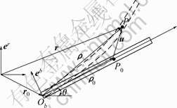
Fig.1 Dynamic model of beam undergoing large overall motions
r=r0+A��=r0+A(��0+u) (1)
where 
 and A is a matrix transforming a vector of eb to
Differentiating Eqn.(1) yields
 (2)
(2)
where  The differentiation of Eqn.(2) leads to
 (3)
(3)
In case that the coupling effect between longitudinal and transverse deformations is taken into account, the deformation of an arbitrary point on the beam can be expressed as follows [10]:
 (4)
(4)
where  represent the axial deformation
and transverse deformation, and 
represents the coupling deformation. Using the finite element technique, w can be discretized as follows:
 (5)
(5)
where  is the element shape function matrix, and pk is the element nodal deformation coordinate matrix. Substituting Eqn.(5) into Eqn.(4), one obtains
 (6)
(6)
where p is the global nodal deformation coordinate matrix, N=NkBk is the shape function matrix, Bk is Boole indicated matrix, and H is the coupling shape function that is given by

 (7)
(7)
3 Dynamic equations
The application of virtual work principle leads to
 (8)
(8)
where T is the kinetic energy of the beam, U is the elastic potential energy of the beam, and  is the virtual work of the external force.
3.1 Variation of deformation energy
Based on geometric nonlinear relationship, the axial normal strain of the beam may be expressed as
 (9)
(9)
where  is the strain generated by axial deformation,
  is the strain generated by transverse bending deformation. For the linear elastic material, the normal stress of the beam with small strain can be expressed as
 (10)
(10)
where E represents elastic modulus. The deformation energy of the beam is given by
 (11)
(11)
The variation of the deformation energy is given by
 (12)
(12)
where K is the global stiffness matrix given by

 (13)
(13)
3.2 Variation of kinetic energy and virtual work of external force
The kinetic energy of the beam may be expressed as
 (14)
(14)
The variation of the kinetic energy of the beam can be written as
 (15)
(15)
where  and
and  can be obtained by substituting Eqn.(6) into Eqns.(2) and (3), respectively. Assuming that the external force f acted on the beam is a distributed force, the coordinate in the frame
  is represented by
  and f in the frame
  is f=Af t, and then the virtual work done by the external force is given by
 (16)
(16)
3.3 Complete geometric nonlinear dynamic equations
Substituting Eqns.(12), (15), (16) into Eqn.(8), the rigid-flexible coupling dynamic equations for an elastic beam can be obtained as
 (17)
(17)
where  represents the generalized
coordinate of the system,  represents Jacobi matrix of constraint equation, �� represents the matrix of the Lagrange multiplier,
  represents the right term of the acceleration constraint equation, M represents the generalized mass matrix and Q represents the generalized force matrix, which are given by
 (18)
(18)
where
 (19)
(19)
 (20)
(20)
 (21)
(21)


 (22)
(22)

 (23)
(23)

 (24)
(24)

 (25)
(25)


 (26)
(26)


 (27)
(27)
where 

 In case that the body force coordinate vector f is constant, the terms related to the body force in the generalized force matrix can be given by
 (28)
(28)
 (29)
(29)
 (30)
(30)
In Eqns.(19-30), the terms without underline are remained in ZOAC model, and the terms with underline are remained in FOAC model, and the terms with double underline are remained in the present complete model. The constant value or constant matrix are given by
 (31)
(31)
 (32)
(32)
 (33)
(33)

 (34)
(34)

 (35)
(35)
 (36)
(36)
 (37)
(37)
 (38)
(38)

 (39)
(39)


 (40)
(40)
4 Numerical simulations
As shown in Fig.2, the beam is assumed to rotate in X0Y0 plane around Z0. It is a typical test problem which has been used in many researches to investigate the effect of dynamic stiffening or geometric stiffening. The dynamic behavior of an elastic beam with prescribed rotation and free rotation is investigated in this section.
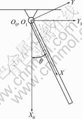
Fig.2 Dynamic model of rotating elastic beam
4.1 Effect of high-order deformation terms
The overall rotation law of the beam is given as follows [3]:
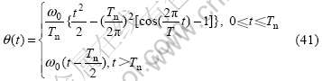
where ��0 is the steady state of the angular velocity, and Tn is the time at which the angular velocity reaches its constant value. The properties of the beam are given as follows: mass density ��=2.767��103 kg/m3, beam length L=1.800 m, area moment of inertia I=1.302��10-10 m4, cross-section area A=2.500��10-4 m2, modulus of elasticity E=68.95 GPa. Three values of the angular velocity, ��0=1, 4, 15 rad/s, are used in the simulation, where the value of Tn is 15 s.
As shown in Fig.3, the beam is discretized with 16 elements in computation. Fig.3(a) shows that the results obtained by the different models agree well in case that the rotation velocity of the beam is low. Fig.3(b) shows that with the increase of the angular velocity, the result obtained by ZOAC model is divergent, whereas the results obtained by the present model and the FOAC model are still stable. As shown in Fig.3(c), when the rotating speed further increases to 15 rad/s, the large deformation appears (tip transverse deformation is more than 1/10 of the length of the beam). It is shown that erroneous results are obtained by using ZOAC model. Comparison of the results obtained by FOAC model and the present model shows that a significant error can be found by using FOAC model in the case of large deformation.
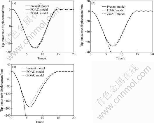
Fig.3 Tip transverse displacement with prescribed motion: (a) ��0=1 rad/s; (b) ��0=4 rad/s; (c) ��0=15 rad/s
4.2 Effect of high-order deformation velocity terms
A single flexible pendulum under the effect of the gravity is shown in Fig.2. To observe the instance of small deformation, the area moment of inertia is given by I=2.604��10-10 m4, and the other properties of the beam are as same as those of the beam in section 4.1. The initial condition of the system is ��=��/2 rad and  0 rad/s without elastic deformation or deformation velocity.
As shown in Fig.4, although the elastic deformation is small, erroneous results are obtained by using FOAC model when the elastic deformation velocity is relatively large. The reason is that the coupling deformation velocity  is not a small quantity compared with the velocity of large overall motion when the elastic deformation velocity is large. However, some high-order terms related to coupling deformation
  and its velocity are neglected in FOAC model, which are the terms with double underline in Eqns.(22-27), therefore, the error or wrong solution is obtained when the deformation or deformation velocity is large. It is shown that the correct solutions can always be obtained by using the present model with the inclusion of the high-order terms related to coupling deformation and its velocity.
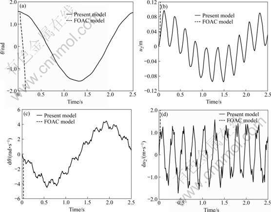
Fig.4 Dynamic response of beam: (a) Overall angle displacement; (b) Tip transverse deformation; (c) Overall angle velocity; (d) Tip transverse deformation velocity
Since the single pendulum with gravity is a conservative system, the sum of the energy components must remain constant, that is T+Ue+Ug=const, where T is the kinetic energy, Ue is the strain energy, and Ug is the potential energy of gravity. As shown in Fig.5, the results present that the total energy of the system remains constant, which verifies the validity of the present method for rigid-flexible coupling dynamics of an elastic beam.
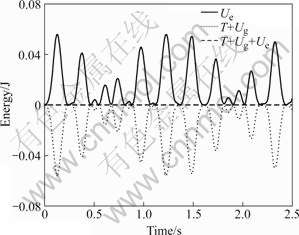
Fig.5 Energy of flexible beam
5 Conclusions
(1) The ZAOC model fails to deal with the dynamic problem of flexible beam with high rotating velocity because the coupling deformation terms are not taken in account.
(2) The FAOC model based on assumption of small deformation can be successfully used to solve the dynamic stiffening problem. However, due to the neglect of some high-order terms related to coupling deformation and its velocity, the FOAC model is not suitable when the deformation or deformation velocity is relatively large.
(3) The correct solutions can always be obtained by using the present model for the high-order terms related to coupling deformation, and regardless of the deformation or deformation velocity is large or small, and the overall rotation velocity is high or low. Furthermore, the validity of the present dynamic model is verified by the principle of conservation of energy.
References
[1] HONG Jia-zhen. Computational dynamics of multibody system [M]. Beijing: High Education Press, 1999. (in Chinese)
[2] TANG Hua-ping, TANG Chun-xi, YIN Chen-feng. Optimization of actuator/sensor position of multi-body system with quick startup and brake [J]. Journal of Central South University of Technology, 2007, 14(6): 803-807.
[3] KANE T, RYAN R. BANERJEE A. Dynamics of a cantilever beam attached to a moving base [J]. Journal of Guidance, Control and Dynamics, 1987, 10: 139-151.
[4] MAYO J, DOMINGUEZ J. Finite element geometrically nonlinear dynamic formulation of flexible multibody systems using a new displacements representation [J]. Journal of Vibration and Acoustics, 1997, 119: 573-581.
[5] YOO H H, CHUNG J, CHUANG J. Equilibrium and modal analyses of rotating multibeam structures employing multiple reference frames [J]. Journal of Sound and Vibration, 2007, 302: 789-805.
[6] LIA A Q, LIEW K M. Non-linear substructures approach for dynamic analysis of rigid-flexible multibody system [J]. Computer Methods in Applied Mechanics and Engineering, 1994, 114: 379- 396.
[7] SHABANA A A, MIKKOLA A M. Use of the finite element absolute nodal coordinate formulation in modeling slop discontinuity [J]. Trans ASME J Mech Des, 2003, 125: 342-350.
[8] SUGIYAMA H, GERSTMAY S, SHABANA A A, Deformation modes in the finite element absolute nodal coordinate formulation [J]. Journal of Sound and Vibration, 2006, 298: 1129-1149.
[9] JIANG Li-zhong, HONG Jia-zhen. Coupling dynamics of the elastic beam with translation [J]. Chinese Quarterly of Mechanics, 2002, 23(4): 450-454. (in Chinese)
[10] LIU Jin-yang. Study of dynamic modeling theory of rigid-flexible coupling system [D]. Shanghai: Department of Engineering Mechanics, Shanghai Jiao Tong University, 2000. (in Chinese)
[11] YANG Hui, HONG Jia-zhen, YU Zheng-yue. Dynamics modeling of a flexible hub-beam system with a tip mass [J]. Journal of Sound and Vibration, 2003, 266(4): 759-774.
[12] LIU Jin-yang, HONG Jia-zhen. Geometric stiffening effect on rigid-flexible coupling dynamics of an elastic beam [J]. Journal of Sound and Vibration, 2004, 278(4/5): 1147-1162.
[13] CAI G P, LIM C W. Optimal tracking control of a flexible hub�Cbeam system with time delay [J]. Multibody System Dynamics, 2006, 16: 331-350.
[14] DONG Xing-jian, MENG Guang, CAI Guo-ping. Dynamic modeling and analysis of a rotating flexible beam [J]. Journal of Vibration Engineering, 2006, 19(4): 488-493. (in Chinese)
[15] HUANG You-an, DENG Zi-chen, YAO Lin-xiao. Dynamic analyze of a rotating rigid-flexible coupled smart structure with large deformation [J]. Applied Mathematics and Mechanics, 2007, 28(10): 1203-1212.
Foundation item: Project(10772113) supported by the National Natural Science Foundation of China
Received date: 2008-05-15; Accepted date: 2008-08-26
Corresponding author: LIU Zhu-yong, PhD; Tel: +86-21-34206496; E-mail: zhuyongliu@hotmail.com
(Edited by YANG You-ping)

