J. Cent. South Univ. (2016) 23: 2972-2983

DOI: 10.1007/s11771-016-3361-0

Limit equilibrium method for slope stability based on assumed stress on slip surface

DENG Dong-ping(邓东平), ZHAO Lian-heng(赵炼恒), LI Liang(李亮)

School of Civil Engineering, Central South University, Changsha 410075, China

Central South University Press and Springer-Verlag Berlin Heidelberg 2016

Abstract: In the limit equilibrium framework, two- and three-dimensional slope stabilities can be solved according to the overall force and moment equilibrium conditions of a sliding body. In this work, based on Mohr-Coulomb (M-C) strength criterion and the initial normal stress without considering the inter-slice (or inter-column) forces, the normal and shear stresses on the slip surface are assumed using some dimensionless variables, and these variables have the same numbers with the force and moment equilibrium equations of a sliding body to establish easily the linear equation groups for solving them. After these variables are determined, the normal stresses, shear stresses, and slope safety factor are also obtained using the stresses assumptions and M-C strength criterion. In the case of a three-dimensional slope stability analysis, three calculation methods, namely, a non-strict method, quasi-strict method, and strict method, can be obtained by satisfying different force and moment equilibrium conditions. Results of the comparison in the classic two- and three-dimensional slope examples show that the slope safety factors calculated using the current method and the other limit equilibrium methods are approximately equal to each other, indicating the feasibility of the current method; further, the following conclusions are obtained: 1) The current method better amends the initial normal and shear stresses acting on the slip surface, and has the identical results with using simplified Bishop method, Spencer method, and Morgenstern-Price (M-P) method; however, the stress curve of the current method is smoother than that obtained using the three abovementioned methods. 2) The current method is suitable for analyzing the two- and three-dimensional slope stability. 3) In the three-dimensional asymmetric sliding body, the non-strict method yields safer solutions, and the results of the quasi-strict method are relatively reasonable and close to those of the strict method, indicating that the quasi-strict method can be used to obtain a reliable slope safety factor.

Key words: two-dimensional slope; three-dimensional slope; limit equilibrium analysis; normal stress; shear stress; safety factor

1 Introduction

The limit equilibrium method [1-4] is commonly used for analyzing slope stability in actual engineering. Generally, on dividing the two-dimensional (or three- dimensional) sliding body into some vertical slices (or columns) [5], different limit equilibrium methods [6-8] are established on a basis of the different assumptions of the inter-slice (or inter column) forces and the force (or moment) equilibrium conditions, such as Swedish method, simplified Bishop method, Spencer method and Morgenstern-Price (M-P) method. These methods have been proven to be feasible and are widely adopted [9-11]. However, for most of the traditional limit equilibrium methods, several iterations should be undergone to solve the slope safety factor, and the results may not even converge, particularly for the strict limit equilibrium solution.

BELL [12] proposed a new method to establish the formula for the slope safety factor by assuming the distribution of the normal stresses acting on a slip surface. This method could solve the overall force and moment equilibrium equations of a sliding body to yield an analytical solution of the slope safety factor, compensating for the shortcomings of the calculation convergence in the conventional methods. Thereafter, ZHU [13] and ZHENG [14] established two- and three-dimensional calculation methods for the slope stability on the basis of this concept. However, the methods proposed by ZHU [13, 15-17] and others need to typically solve unitary multiple equations on the slope safety factor, and this way is particularly troublesome to calculate the strict limit equilibrium solution of a three- dimensional slope, which consists of unitary six square equations.

In contrast to the studies conducted by BELL [12], ZHU and LEE [13] and ZHENG and THAM [14], which assume only the distribution of the normal stress acting on a slip surface, this work considers both the assumptions of the normal and shear stresses acting on a slip surface based on Mohr-Coulomb (M-C) strength criterion and the initial normal stress without considering the inter-slice forces (or inter-column) in a infinitesimal slice (or column). Same dimensionless variables are adopted to assume the normal and shear stresses and they have the same number with the force and moment equilibrium conditions of the sliding body. Thus, these variables can be obtained by solving limit equilibrium equations, and subsequently, the normal stress, shear stress, and safety factor for the overall slope stability are also obtained using the stresses assumptions and M-C strength criterion. As compared with the methods proposed by ZHU et al [13, 15-17], the current method yields some multiple linear equations for these variables that are convenient to solve. The feasibility of the current method has been verified by applying it to a few classic two- and three-dimensional slope examples, and it can be used to quickly obtain a reliable slope safety factor. Furthermore, the current method can be used to analyze the slope stability under complex conditions or with three- dimensional asymmetric sliding bodies. Moreover, three calculation methods, namely, a non-strict method, quasi- strict method, and strict method, are established and applied on the basis of the different numbers of force and moment equilibrium equations that are satisfied in a three-dimensional sliding body.

2 Two-dimensional slope stability analysis

2.1 Basic theory

Figure 1 shows a slope under general conditions, where P₀ and P_n are the toe and top points of the slope, respectively. P₀ is considered the origin to establish the xy-axis coordinate system, and A and B are the lower and upper sliding points of the slip surface, respectively. The equations for the slip surface and the slope outline are y= s(x) and y=g(x), respectively. The infinitesimal slice abcd with width dx is separated to analyze the forces, and portion ebcf is below the saturation line. In slice abcd, the gravity is wdx; the horizontal and vertical forces acting on the slope surface are q_xdx and q_ydx, respectively; the normal and shear forces acting on the slip surface are σdx/cosα and τdx/cosα, respectively; the pore water force is udx/cosα; and the horizontal and vertical seismic forces are k_Hwdx and k_Vwdx, respectively, where k_H and k_V are the horizontal and vertical seismic coefficients, respectively.

Without considering the inter-slice forces in the infinitesimal slice, the force equilibrium conditions in the x- and y-directions can be given as

                      (1a)

                  (1b)

Fig. 1 Stress analysis of infinitesimal slice in two- dimensional slope

where σ₀ and τ₀ are the normal and shear stresses acting on the slip surface without considering inter-forces, respectively; , and α is the horizontal inclination angle of the slip surface in the infinitesimal slice.

Solving Eq. (1), the normal stress σ₀ is expressed as

            (2)

However, the actual normal stress acting on the slip surface should be determined by taking the effect of the inter-slice forces into account; thus, the normal stress σ₀ obtained using Eq. (2) must be amended. In the case of a two-dimensional slope stability analysis, the normal stress σ is calculated using:

                                   (3)

where λ₁ is the dimensionless variable.

In the slope stability analysis, the shear stress τ acting on the slip surface can be derived from the M-C strength criterion as

                          (4)

where c is the soil cohesion; φ is the soil internal friction; and F_s is the slope safety factor.

According to Eq. (4), the shear stress τ can be calculated from the sum of the following two parts: part I is (c–utanφ)/F_s, and part Ⅱ is σtanφ/F_s. If we let λ₂=1/F_s and λ₃=λ₁/F_s, the formula for τ will then be expressed as

                             (5)

where λ₂ and λ₃ are the dimensionless variables, τ₀₁=c– utanφ, and τ₀₂=σ₀tanφ.

Three variables λ₁, λ₂, and λ₃ are included in Eqs. (3) and (5) for calculating the normal and shear stresses, and they can be solved by applying three limit equilibrium equations of a two-dimensional sliding body. As shown in Fig. 1, the x- and y-direction force equilibrium equations and moment equilibrium equation around a point (x_c, y_c) are given as

              (6a)

            (6b)

                  (6c)

Substituting Eqs. (6a) and (6b) into Eq. (6c), Eq. (6c) can be abbreviated as

              (7)

Substituting Eqs. (3) and (5) into Eqs. (6a), (6b), and (7), the linear ternary equations of variables λ₁, λ₂, and λ₃ are deduced as

                       (8)

where a_ij and b_i are the calculation parameters, and their formulas are listed in Table 1.

Table 1 Calculation parameters for two-dimensional slope stability analysis

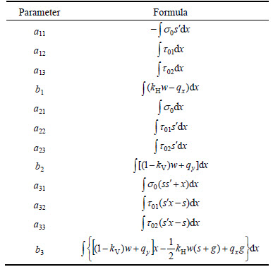
Solving Eq. (8), we can obtain variables λ₁, λ₂, and λ₃, and the normal and shear stresses are also determined according to Eqs. (3) and (5), respectively.

2.2 Calculation of safety factor for two-dimensional slope

In M-C strength criterion expressed by Eq. (4), the slope safety factor can be defined as the ratio of the failure shear force to the shear force acting on a slip surface. Therefore, by summing Eq. (4) over the slip surface, the safety factor F_s for the two-dimensional slope is derived as

                  (9)

3 Three-dimensional slope stability analysis

3.1 Basic theory

Figure 2(a) shows the three-dimensional slip body under general conditions. The neutral plane is the axisymmetric surface of a three-dimensional symmetric sliding body or the main slip surface of a three- dimensional asymmetric sliding body. An xz-axis coordinate system is established by setting the slope toe point of the neutral plane as the origin, and the y-axis direction is determined on the basis of the right-hand rule. The equations of the slip surface and the slope outline are z=s(x, y) and z=g(x, y), respectively. Taking the neutral plane as the interface, we divide the three- dimensional sliding body into the left and right parts, where the widths of the three-dimensional sliding body and its left- and right-half parts are W, w₁, and w₂, respectively. Figure 2(b) shows the force analysis of a infinitesimal column with x-width dx and y-width dy. In the infinitesimal column, the gravity is wdxdy; the x-, y-, and z-direction external loads are q_xdxdy, q_ydxdy, and q_zdxdy, respectively; the normal and shear forces acting on the three-dimensional slip surface are σΔdxdy and τΔdxdy, respectively; the pore water force is uΔdxdy; and the horizontal and vertical seismic forces are k_Hwdxdy and k_Vwdxdy, respectively.

Unlike in the case of the two-dimensional slope stability analysis, in the three-dimensional slope stability analysis, the directions of the normal stress σ and shear stress τ need to be analyzed and calculated. For facilitating to analyze, some parameters are defined as the x-, y-, and z-directional cosines of the normal stress and respectively, and the x-, y-, and z-directional cosines of the shear stress and respectively. In the infinitesimal column, the directional cosines of the normal stress can be easily determined as

                                 (10a)

                                (10b)

                                   (10c)

where and α_x and α_y are the horizontal inclination angles of the slip surface of the infinitesimal column in the xz and yz

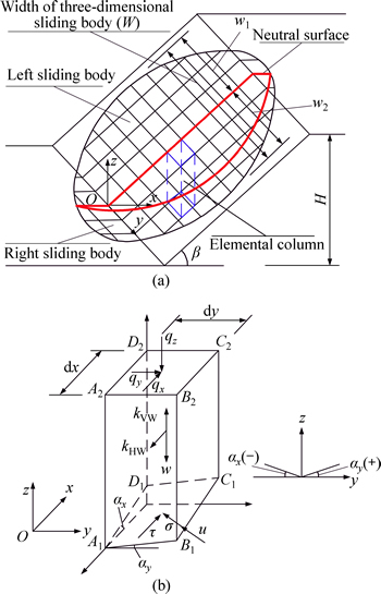
Fig. 2 Stress analysis of infinitesimal column in three- dimensional slope

planes, respectively.

It should be noted that the directional cosines of the normal and shear stresses obey the following relationships:

                     (11a)

                      (11b)

In the three-dimensional slope stability analysis, the direction of the shear stress is usually assumed to be parallel to the neutral plane [15-17]; thus, the directional cosine is given as

                                    (12)

By substituting Eqs. (10) and (12) into Eq. (11) and noting that is always positive, the directional cosines and are calculated as

                        (13a)

                      (13b)

As shown in Fig. 2(b), the x-, y-, and z-direction force equilibrium conditions without considering the inter-column forces in the infinitesimal column are given as

                  (14a)

                       (14b)

              (14c)

where σ₀ and τ₀ are the normal and shear stresses without considering the inter-column forces, respectively.

Combining Eqs. (14a) and (14c), the normal stress σ₀ can be calculated as

          (15)

Likewise the two-dimensional slope stability analysis, the normal stress σ₀ shows also some differences with the actual normal stress σ because the effect of the inter-column forces is not taken into consideration in the three-dimensional slope stability. For the two-dimensional calculation method, the amending formula is shown by Eq. (3). However, given that six limit equilibrium conditions exist for a three-dimensional sliding body, the two-dimensional amending formula should be extended and the normal stress σ acting on the three-dimensional slip surface is calculated as

                      (16)

where λ₁ and λ₂ are the dimensionless variables; y is the y-axis coordinate of the calculated point; and W is the width of the three-dimensional sliding body.

Failure of the three-dimensional slope also obeys the M-C strength criterion, and the calculation modes of the shear stress acting on the two- and three-dimensional slip surfaces are consistent. According to the numbers of the limit equilibrium conditions in the three-dimensional sliding body and substituting Eq. (16) into Eq. (4), we can assume the shear stress acting on the three- dimensional slip surface as

              (17)

where λ₃–λ₆ are the dimensionless variables, and τ₀₁ and τ₀₂ are the same with Eq. (5).

In a three-dimensional sliding body, the x-, y-, and z-direction force equilibrium equations and moment equilibrium equations around the x-, y-, and z-axes about a point (x_c, y_c, z_c) are given as

           (18a)

                 (18b)

            (18c)

                   (18d)

 (18e)

                    (18f)

Substituting Eqs. (18a)-(c) into Eqs. (18d), (18e), and (18f), Eqs.(18d), (18e), and (18f) are respectively abbreviated as

        (19a)

      (19b)

                    (19c)

Substituting Eqs. (16) and (17) into Eqs. (18a)–(c) and (19), the linear equations of the six variables λ₁–λ₆ can be obtained as

              (20)

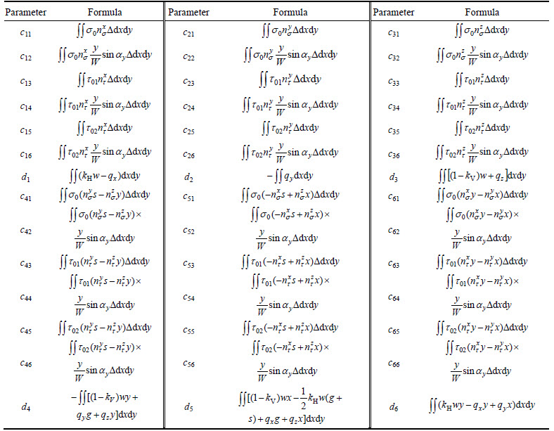
where c_ij and d_i are the calculation parameters, and their formulas are listed in Table 2.

Solving Eq. (20), we determine variables λ₁–λ₆, and the normal and shear stresses acting on the three-dimensional slip surface can be obtained by substituting these variables into Eqs. (16) and (17).

Table 2 Calculation parameters for three-dimensional slope stability analysis

3.2 Calculation of safety factor for three-dimensional slope

According to the M-C strength criterion, the safety factor of the three-dimensional slope has the same definition as that of the two-dimensional slope. Therefore, the safety factor of the three-dimensional slope can be calculated by extending Eq.(4) and is given as

                (21)

3.3 Slope stability analysis on different types of three-dimensional sliding bodies

In the three-dimensional slope stability analysis, the sliding body may either be symmetric under simple conditions or asymmetric under complex conditions. In the case of three-dimensional symmetric sliding bodies, the y-direction force equilibrium equation and moment equilibrium equations around the x- and z-axes are satisfied; thus, the remaining three equations can only be adopted to solve the slope stability. Then, we let λ₂=0, λ₄=0, and λ₆=0, and variables λ₁, λ₃, and λ₅ are calculated using Eqs. (18a), (18b), and (19b). Meanwhile, the normal stress σ, shear stress τ, and slope safety factor F_s can be obtained on the basis of these known variables.

In the stability analysis of a three-dimensional asymmetric sliding body, the six limit equilibrium conditions shown in Eqs. (18) exist, and three calculation methods can be typically adopted. The three methods, namely, the non-strict method, quasi-strict method, and strict method, are derived by using the different numbers of limit equilibrium conditions that the three-dimensional sliding body should satisfy, and their detailed calculation processes are listed in Table 3.

By solving the relationship conditions shown in Table 3, we can determine the variables for the three methods, and the normal stress σ, shear stress τ, and slope safety factor F_s can also be obtained.

4 Calculation and comparative analysis

4.1 Stability analysis of two-dimensional slope

Example 1 [18]: Slope height H=10 m and slope ratio=1:2; the soil parameters are as follows: natural unit gravity γ=20.0 kN/m³, cohesion c=3.0 kPa, and internal friction angle φ=19.6°.

Example 2 [18]: Slope height H=10 m and slope ratio=1:2; the soil parameters are as follows: natural unit gravity γ₁=19.5 kN/m³, cohesion c₁=0.0 kPa, and internal friction angle φ₁=38.0° for soil #1; natural unit gravity γ₂=19.5 kN/m³, cohesion c₂=5.3 kPa, and internal friction angle φ₂=23.0° for soil #2; natural unit gravity γ₃=19.5 kN/m³, cohesion c₃=7.2 kPa, and internal friction angle φ₃=20.0° for soil #3.

4.1.1 Comparison of normal and shear stresses acting on two-dimensional slip surface

An xy-axis coordinate system is established by setting the slope toe point as the origin. A and B are the lower and upper sliding points of the slip surface, respectively. Two types of slip surfaces, i.e., a circular slip surface and an arbitrary curved slip surface, are used to analyze the slope stability. When the circular slip surface is adopted, the circular slip surface radius is R=30 m and the coordinates of points A and B are (0 m, 0 m) and (22 m, 10 m), respectively, for example 1; the circular slip surface radius is R=18 m and the coordinates of points A and B are (0 m, 0 m) and (22 m, 10 m), respectively, for example 2. The normal and shear stresses calculated using the current method, Swedish method, Simplified Bishop method, Spencer method, and M-P method are compared, and the results of the comparison are shown in Figs. 3-4. Because the normal and shear stresses of Spencer method have small difference with that of M-P method, both of the results obtained by these two methods are shown in Fig. 3(c) for example 1 and Fig. 4(c) for example 2.

When the arbitrary curved slip surface, proposed by DENG et al [19], is adopted, the coordinates of points A and B are (0 m, 0 m) and (22 m, 10 m), respectively, n=100, x₀= (x_B–x_A)/n, and α₀=0° for example 1, where, x_A and x_B are respectively the x-axes coordinates of points A and B, n is the number of plotlines, x₀ is the horizontal width of the first plotline, α₀ is the horizontal inclination angle of the first plotline, and it is positive when α₀ is measured in the clockwise direction; the coordinates of points A and B are (0 m, 0 m) and (22 m, 10 m), respectively, n=100, x₀=(x_B–x_A)/n, and α₀=0° for example 2. The normal and shear stresses calculated using the current method, Spencer method, and M-P method are compared, and the results of this comparison are shown in Fig. 5. Likewise, because the normal and shear stresses of Spencer method have small difference with that of M-P method, both of the results obtained by these two methods are shown in Fig. 5.

Table 3 Calculation methods for three-dimensional asymmetric sliding body

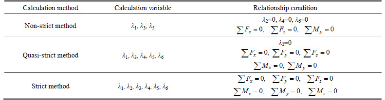
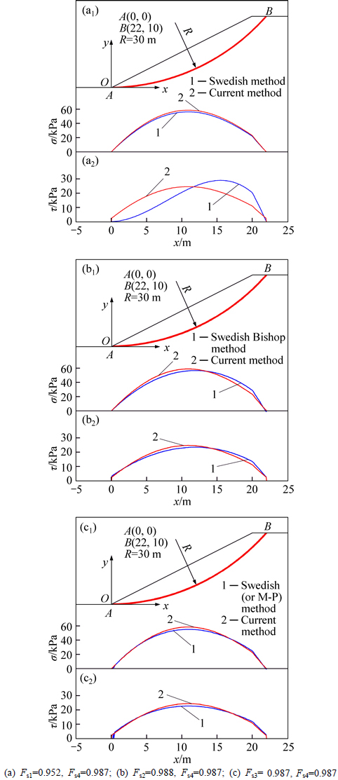
Fig. 3 Contrast of stress on circular slip surface in example 1:(Noting that F_s1 is the slope safety factor of Swedish method, F_s2 is the slope safety factor of simplified Bishop method, F_s3 is the slope safety factor of Spencer (or M-P) method and F_s4 is the slope safety factor of the current method)

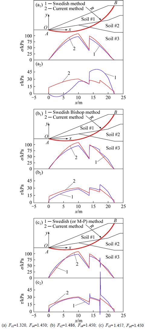
Fig. 4 Contrast of stress on circular slip surface in example 2:(Noting that F_s1 is the slope safety factor of Swedish method, F_s2 is the slope safety factor of simplified Bishop method, F_s3 is the slope safety factor of Spencer (or M-P) method and F_s4 is the slope safety factor of the current method)

From Figs. 3-5, it is observed that the normal and shear stresses obtained using the current method are approximately equal to those calculated using simplified Bishop method, Spencer method, and M-P method and that the current method better amends the initial normal stress σ₀ without considering the effect of inter-slice forces, as observed in the case of the results of Swedish method. Additionally, the normal and shear stress curves obtained using the current method are smoother than those obtained using Spencer method and M-P method. Further, in examples 1 and 2, compared with the conventional limit equilibrium methods, the shear stresses in both end sides obtained by the current method are relatively higher, the reason of which is that the current method is established on the basis of the overall limit equilibrium conditions of a sliding body.

4.1.2 Comparison of critical slip surface

In order to verify the feasibility of the current method, the circular and arbitrary curved slip surfaces are also adopted to analyze the stability of slopes in examples 1–2. The minimum slope safety factor and critical slip surface for the two examples are given in Table 4 and Figs. 6-7. From this table and the figures, it can be inferred that the results of the current method are in quite good agreement with those of simplified Bishop method, Spencer method, and M-P method. It should be noted that the current method can satisfy all the limit equilibrium conditions of a sliding body, owing to which its results are larger than those of Swedish method; further, the strictness of the current method has been illustrated.

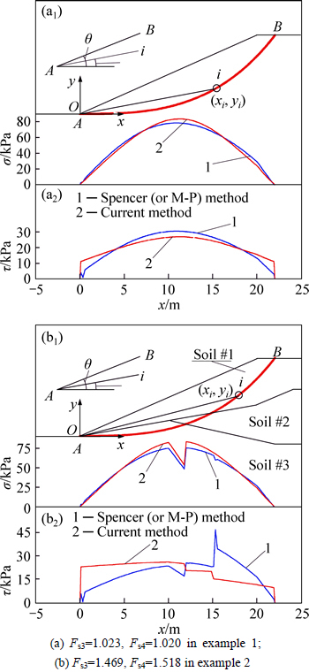
Fig. 5 Contrast of stress on arbitrary curved slip surface in slope examples (Noting that F_s3 is the slope safety factor of Spencer (or M-P) method and F_s4 is the slope safety factor of the current method):

4.2 Three-dimensional slope stability analysis

Example 3: A homogeneous slope is shown in Fig. 8(a), with slope height H=40 m, slope angle β=45°. In the soil, natural unit gravity γ=22 kN/m³, cohesion c= 30 kPa, and internal friction angle φ=30°. The slip surface is assumed to be a rotating ellipsoid described by equation with x₀=0 m,z₀=40 m, a=40 m, and where W is the width of the sliding body. The xyz-axis coordinate system is established by setting the slope toe point of the neutral plane as the origin. A and B are the lower and upper sliding points of the two-dimensional main slip surface in the three-dimensional sliding body, respectively. The coordinates of points A and B are (0 m, 0 m, 0 m) and (40 m, 0 m, 40 m), respectively, and the two-dimensional main slip surface is circular with radius R=40 m.

Example 4 [20]: Another homogeneous slope is shown in Fig. 8(b), with slope height H=12.2 m, slope ratio=1:2. In the soil, natural unit gravity γ=19.2 kN/m³, cohesion c=29.3 kPa, and internal friction angle φ=20°. A three-dimensional arbitrary curved slip surface, proposed by DENG et al [21], is adopted to analyze the slope stability.

Table 4 Contrast of minimum slope safety factor in two-dimensional slope stability analysis

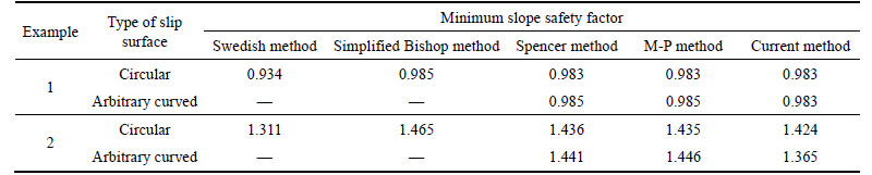
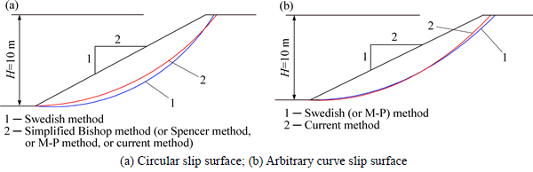
Fig. 6 Contrast of critical slip surface in example 1:

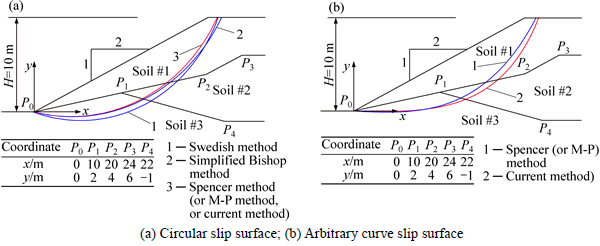
Fig. 7 Contrast of critical slip surface in example 2:

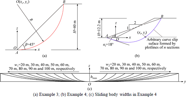
Fig. 8 Two-dimensional graphics of three-dimensional slip surface in slope examples:

4.2.1 Three-dimensional symmetric sliding body

In Example 3, the ratio of the sliding body width W to the slope height H was assumed to be 1, 2, 3, 4, 5, 6, 7, and 8. The slope safety factor is calculated, and the results of which are shown in Fig. 9(a). From Fig. 9(a), it can be inferred that the results of the current method are less than those of the improved three-dimensional safety factor method [22] and are larger than those of the three-dimensional ordinary column method [23]. Further, the results of the current method are in good agreement with those of the three-dimensional simplified Bishop method [24], three-dimensional simplified Janbu method [25], three-dimensional Spencer method [20], three- dimensional M-P method [26], and three-dimensional Sarma method [27], with a difference of only approximately 4%.

In Example 4, the xyz-axis coordinate system is also established by setting the slope toe point of the neutral plane as the origin, and the parameters of the three-dimensional arbitrary curved slip surface are given as n=50, m=100, x_A=-5.71 m, z_A=0 m, x_B=28.72 m, z_B= 12.2 m, x₀=(x_B-x_A)/n, y₀₁=w₁/m, y₀₂=w₂/m, α₀=18°, α₀₁= 0°, and α₀₂=0°, where (x_A, z_A) and (x_B, z_B) are respectively the x- and z-axis coordinates of points A and B, n is the number of rows parallel to the y-axis and 2m is the number of columns parallel to the x-axis, x₀ is the horizontal width of the first row parallel to the y-axis, y₀₁ and y₀₂ are respectively the horizontal widths of the first column parallel to the x-axis in the left and right sliding bodies, α₀ is the horizontal inclination angle of the first plotline in the first column parallel to the x-axis, and α₀₁ and α₀₂ are respectively the horizontal inclination angles of the first plotline in the first row of the left and right sliding bodies parallel to the y-axis. The slope safety factor is calculated for different values of widths W of a three-dimensional sliding body shown in Fig. 8(c), such as for 40 m, 60 m, 80 m, 100 m, 120 m, 140 m, 160 m, 180 m, and 200 m, and the results of this calculation are shown in Fig. 9(b). As shown in Fig. 9(b), the safety factor of a two-dimensional main slip surface is also obtained by the two-dimensional calculation method.

From Fig. 9, it can be inferred that the current method yields reasonable results, which are approximately equal to those of the other methods, and the safety factor of a three-dimensional slip surface tends to that of a two-dimensional main slip surface with an increase in the width of the three-dimensional sliding body.

4.2.2 Three-dimensional asymmetric sliding body

Example 4 assumes three-dimensional asymmetric sliding bodies. In the case of a three-dimensional asymmetric sliding body, the widths or curved surfaces of the left and right parts of the sliding body differ from each other. The aforementioned three calculation methods, namely, the non-strict method, quasi-strict method, and strict method, are adopted to analyze the stability of a three-dimensional asymmetric sliding body.

As shown in Fig. 10(a), the widths of the left and right parts of the sliding body differ from each other, and other parameters of the three-dimensional arbitrary curved slip surface are identical to those considered in example 4. It should be noted that the width of the right part is w₂=50 m, and the width of the left part is w₁=50 m, 60 m, 70 m, 80 m, 90 m, and 100 m, respectively. The results of the abovementioned three calculation methods are listed in Table 5.

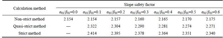
As shown in Fig. 10(b), curved surfaces of the left and right parts of the sliding body differ from each other. Apart from angle α₀₂, other parameters of the three- dimensional arbitrary curved slip surface are identical to those considered in example 4. The results of the three calculation methods are listed in Table 6, where angle α₀₁=0.0β₀₁, 0.15β₀₁, 0.3β₀₁, 0.45β₀₁, 0.6β₀₁, 0.75β₀₁, and 0.9β₀₁, respectively; the left part width w₁=50 m, and the right part width w₂=50 m.

From Tables 5 and 6, it can be inferred that the results of the non-strict method are smaller than those of the two other methods, and the results of the quasi-strict method are approximately equal to those of the strict method. Thus, the non-strict method yields safer results and the simplified quasi-strict method yields a reasonable slope safety factor.

Fig. 9 Contrast of safety factor for three-dimensional symmetric slip surface

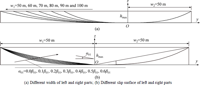
Fig. 10 Three-dimensional asymmetric sliding body (Noting that β₀₁ and β₀₂ are the maximum horizontal inclination angles of the left and right sliding bodies in plane yz, respectively, where β₀₁=arctan (h_max/w₁), β₀₂=arctan (h_max/w₂), and h_max is the maximum vertical depth between the two-dimensional main slip surface and the slope surface):

Table 5 Contrast of slope safety factor in three-dimensional asymmetry sliding body with different widths of left and right parts

Table 6 Contrast of slope safety factor in three-dimensional asymmetry sliding body with different slip surfaces of left and right parts

5 Conclusions

1) The normal and shear stresses obtained using the current method are identical to those obtained using simplified Bishop method, Spencer method, and M-P method, and the current method yields a relatively smooth stress curve, indicating that the current method better amends the initial normal stress calculated by Swedish methods. Further, the current method is established on the basis of the overall limit equilibrium conditions, and therefore, its results differ slightly from those of the conventional calculation methods.

2) The current method is suitable for analyzing two- and three-dimensional slope stability. The safety factor and the critical slip surface of the slope calculated using the current method and the other limit equilibrium methods are approximately similar to each other, indicating the feasibility of the current method. Further, the current method can satisfy all the limit equilibrium conditions of a sliding body, therefore it yields stricter solutions than Swedish method.

3) In the case of a three-dimensional slope stability analysis, the non-strict method yields safer solutions and the results of the quasi-strict method are approximately equal to those of the strict method, indicating that the quasi-strict method yields a reliable slope safety factor.

References

[1] LIU S Y, SHAO L T, LI H J. Slope stability analysis using the limit equilibrium method and two finite element methods [J]. Computers and Geotechnics, 2005, 63(1): 291-298.

[2] CHENG Y M, LANSIVAARA T, WEI W B. Two-dimensional slope stability analysis by limit equilibrium and strength reduction methods [J]. Computers and Geotechnics, 2007, 34(3): 137-150.

[3] WEI W B, CHENG Y M, LI L. Three-dimensional slope failure analysis by the strength reduction and limit equilibrium methods [J]. Computers and Geotechnics, 2009, 36(1): 70-80.

[4] ZHU J F, CHEN C F. Search for circular and noncircular critical slip surfaces in slope stability analysis by hybrid genetic algorithm [J]. Journal of Central South University, 2014, 21(1): 387-397.

[5] TAHA M R, KHAJEHZADEH M, ESLAMI M. A new hybrid algorithm for global optimization and slope stability evaluation [J]. Journal of Central South University, 2013, 20(11): 3265-3273.

[6] LAM L, FREDLUND D G. A general limit equilibrium model for three-dimensional slope stability analysis [J]. Canadian Geotechnical Journal, 1993, 30(6): 905-919.

[7] CHENG Y M, YIP C J. Three-dimensional asymmetrical slope stability analysis extension of Bishop’s, Janbu’s, and Morgenstern– Price’s techniques [J]. Journal of Geotechnical and Geoenvironmental Engineering, 2007, 133(122): 1544-1555.

[8] ZHOU X P, CHENG H. Analysis of stability of three-dimensional slopes using the rigorous limit equilibrium method [J]. Engineering Geology, 2013, 160(27): 21-33.

[9] FREDLUND D G, KRAHN J. Comparison of slope stability methods of analysis [J]. Canadian Geotechnical Journal, 1997, 14(3): 429-439.

[10] LESHCHINSKY D, BAKER R, SILVER M L. Three dimensional analysis of slope stability [J]. International Journal for Numerical and Analytical Methods in Geomechanics, 1985, 9(3): 199-223.

[11] ZHU D Y, LEE C F, JIANG H D. Generalized framework of limit equilibrium methods for slope stability analysis [J]. Géotechnique, 2003, 53(4): 377-395.

[12] BELL J M. General slope stability analysis [J]. Journal of the Soil Mechanics and Foundations Division, ASCE, 1968, 94(SM6): 1253-1270.

[13] ZHU D Y, LEE C F. Explicit limit equilibrium solution for slope stability [J]. International Journal for Numerical and Analytical Methods in Geomechanics, 2002, 26(15): 1573-1590.

[14] ZHENG H, THAM L G. Improved Bell’s method for the stability analysis of slopes [J]. International Journal for Numerical and Analytical Methods in Geomechanics, 2009, 33(14): 1673-1689.

[15] ZHU D Y, DING X L, DU J H, DENG J H. Computation of 3D safety factor of asymmetric and rotational slopes [J]. Chinese Journal of Rock Mechanics and Engineering, 2007, 29(8): 1236-1239. (in Chinese)

[16] ZHU D Y, DING X L, LIU H L, QIAN Q H. Method of three-dimensional stability analysis of a symmetrical slope [J]. Chinese Journal of Rock Mechanics and Engineering, 2007, 26(1): 22-27. (in Chinese)

[17] ZHU D Y, QIAN Q H. Rigorous and quasi-rigorous limit equilibrium solutions of 3D slope stability and application to engineering [J]. Chinese Journal of Rock Mechanics and Engineering, 2007, 26(8): 1513-1528. (in Chinese)

[18] Rocscience Inc. Slide verification manual [M]. Toronto: Rocscience Inc, 2003: 8-118.

[19] DENG D P, LI L, ZHAO L H. A new method of sliding surface searching for general stability of slope based on Janbu method [J]. Rock and Soil Mechanics, 2011, 32(3): 891-898. (in Chinese)

[20] ZHANG X. Three-dimensional stability analysis of concave slopes in plan view [J]. Journal of Geotechnical Engineering, ASCE, 1988, 114(6): 658-671.

[21] DENG D P, LI L, ZHAO L H. A new method for searching sliding surface of three-dimensional homogeneous soil slope [J]. Chinese Journal of Rock Mechanics and Engineering, 2010, 29(S2): 3719-3727. (in Chinese)

[22] WANG Y X, DENG H K. An improved method for three-dimensional slope stability analysis [J]. Chinese Journal of Geotechnical Engineering, 2003, 25(5): 611-614. (in Chinese)

[23] HOVLAND H J. Three-dimensional slope stability analysis method [M]. Journal of Geotechnical Engineering Division, 1997, 103(9): 971-986.

[24] HUNGR O. An extension of Bishop’s simplified method of slope stability analysis to three dimensions [J]. Geotechnique, 1987, 37(1): 113-117.

[25] HUNGR O, SALGADO F M, BYRNE P M. Evaluation of a three-dimensional method of slope stability analysis [J]. Canadian Geotechnical Journal, 1989, 26(4): 679-686.

[26] CHEN C F, ZHU J F. A three-dimensional slope stability analysis procedure based Morgenstern-Price method [M]. Chinese Journal of Rock Mechanics and Engineering, 2010, 29(7): 1473-1480. (in Chinese)

[27] DENG D P, LI L. Quasi-rigorous and non-rigorous 3D limit equilibrium methods for generalized-shaped slopes [J]. Chinese Journal of Geotechnical Engineering, 2013, 35(3): 501-511. (in Chinese)

(Edited by YANG Hua)

Foundation item: Project(51608541) supported by the National Natural Science Foundation of China; Project(2015M580702) supported by the Postdoctoral Science Foundation of China; Project(201508) supported by the Postdoctoral Science Foundation of Central South University, China

Received date: 2015-05-27; Accepted date: 2015-08-06

Corresponding author: DENG Dong-ping, Post-doctor; Tel: +86-13975150476; E-mail: dengdp851112@126.com