J. Cent. South Univ. (2017) 24: 2438-2448

DOI: https://doi.org/10.1007/s11771-017-3655-x

Multi-scale regionalization based mining of spatio-temporal teleconnection patterns between anomalous sea and land climate events

XU Feng(徐枫)¹, SHI Yan(石岩)^{2, 3}, DENG Min(邓敏)¹, GONG Jian-ya(龚健雅)^{2, 3},

LIU Qi-liang(刘启亮)¹, JIN Rui(金瑞)¹

1. Department of Geo-informatics, Central South University, Changsha 410083, China;

2. State Key Laboratory of Information Engineering in Surveying (Mapping & Remote Sensing,Wuhan University), Wuhan 430079, China;

3. Collaborative Innovation Center of Geospatial Technology, Wuhan University, Wuhan 430079, China

Central South University Press and Springer-Verlag GmbH Germany 2017

Abstract: Climate sequences can be applied to defining sensitive climate zones, and then the mining of spatio-temporal teleconnection patterns is useful for learning from the past and preparing for the future. However, scale-dependency in this kind of pattern is still not well handled by existing work. Therefore, in this study, the multi-scale regionalization is embedded into the spatio-temporal teleconnection pattern mining between anomalous sea and land climatic events. A modified scale-space clustering algorithm is first developed to group climate sequences into multi-scale climate zones. Then, scale variance analysis method is employed to identify climate zones at characteristic scales, indicating the main characteristics of geographical phenomena. Finally, by using the climate zones identified at characteristic scales, a time association rule mining algorithm based on sliding time windows is employed to discover spatio-temporal teleconnection patterns. Experiments on sea surface temperature, sea level pressure, land precipitation and land temperature datasets show that many patterns obtained by the multi-scale approach are coincident with prior knowledge, indicating that this method is effective and reasonable. In addition, some unknown teleconnection patterns discovered from the multi-scale approach can be further used to guide the prediction of land climate.

Key words: climate sequences; anomalous climatic events; spatio-temporal teleconnection patterns; multi-scale regionalization

1 Introduction

The rapid development of earth observation technology makes it possible for easy acquisition of long time series in distinct spatial regions regarding to multiple climate parameters, i.e., climate sequences. In climate sequences, spatio-temporal teleconnection patterns refer to the responding/driving relationships with respect to anomalous climatic events among distinct climate regions (e.g, sensitive marine regions) with large distances [1]. The most well known teleconnection pattern may be the El Southern Oscillation(ENSO) that refers to the effects of a band of sea surface temperatures that are anomalously warm or cold for long period of time that develops off the western coast of South America and causes climatic changes across the tropics and subtropics. Discovery of spatio-temporal teleconnection patterns is helpful for learning from the past and preparing for the future [2]. Some researchers have attempted to discover this kind of pattern by employing statistical methods, such as principal component analysis [3], singular value decomposition [4] and climate network [5, 6]. However, these statistical methods are only useful for discovering a few of the strongest patterns, thus some complex and interesting patterns cannot be captured by these methods [7]. In addition, the statistical methods impose a condition that all discovered singles must be orthogonal to each other, making it difficult to interpret the discovered patterns [8].

To overcome the limitations of statistical methods, spatio-temporal data mining techniques have been developed to explore spatio-temporal teleconnection patterns from massive climate sequences, e,g., spatial clustering and association rules mining [9–11]. Although it is known that spatio-temporal patterns are scale- dependent, the effect of spatial scale is not well handled by existing works, so the unclear scale information will lead to a fact that the obtained knowledge may be misleading or unreliable [12, 13]. Therefore, the purpose of this study is to propose a framework by combining multi-scale regionalization and temporal association rules mining to mine spatio-temporal teleconnection patterns between anomalous sea and land climate events.

2 Related works and methodology of our mining procedure

Many recent studies have been conducted to discover association rules from temporal sequences. These works can be modified or directly used to detect teleconnection patterns from climate sequences. In addition, some hybrid methods combing spatial clustering and temporal association rules mining were further developed to mine spatio-temporal teleconnection patterns. In the following, details of these two kinds of methods will be reviewed.

2.1 Temporal association rules mining methods

Temporal association rule mining methods aim to discover frequent events and association rules from time series. For example, MANNILA et al [14] introduced the concept of sliding time windows to perform this, i.e., the WINEPI and MINEPI methods; DAS et al [15] obtained a series of time intervals from a time series by clustering and then mined association rules among these time intervals; HARMS et al [16] proposed a MOWCATL method, which takes into account time lags between two events; XUE et al [1, 17, 18] shared the core idea of the Apriori algorithm to explore abnormal association patterns among the marine parameters and the ENSO events.

Although these methods can be modified to discover spatio-temporal teleconnection patterns from times series recorded in distinct regions, positive spatial autocorrelation (i.e. adjacent climate sequences generally possess a high degree of similarity) among these regions cannot be considered. Therefore, large number of redundant rules will be discovered because of the positive spatial autocorrelation in climate sequences [2].

2.2 Hybrid methods to mine spatio-temporal teleconnection patterns

In the hybrid methods, discovery of climate zones with similar climatological behaviors plays the key role in handling the effect of positive spatial autocorrelation on teleconnection pattern mining. Spatial clustering techniques are usually used to divide a dataset into climate zones, where objects in the same climate zone are similar and objects in separate climate zones are as different as possible [19]. Thus, the effect of positive spatial autocorrelation on mining teleconnection patterns can be alleviated. Currently, partitioning, hierarchical and density-based clustering methods are commonly used to perform the process of climate zone partitioning [11, 20, 21]. Similarly, climate zones can also be identified by means of community detection from the complex network constructed by the climate sequences [22, 23]. In addition, XUE et al [24] introduced related priori knowledge in climatology to unveil climate zones, e.g., regions affected by widespread processes such as the western Pacific warm pool.

Focusing on the delineated climate zones, correlation analysis (e.g. Pearson correlation coefficient) [7, 25], temporal association rule mining methods (e.g. WINEPI and MINEPI) [14–16], or mutual information [26, 27] can be a sued to identify teleconnection patterns among different climate zones.

Based on the analysis above, one can see that spatial clustering is an effective tool for delineation of climate zones, but the effect of spatial scales on mining teleconnection patterns is not well considered. Here, spatial scale can be measured by the size and number of climate zones [28]. It is known that the size and number of climate zones are usually varied with different clustering methods and parameters. However, the climate zones for discovery of teleconnection patterns are subjectively selected by existing work. Further, the successive detected teleconnection patterns are also subjective and difficult to interpret. To overcome the shortcomings of previous works, it is necessary to develop a new methodology to discover teleconnection patterns from climate sequences.

2.3 A multi-scale regionalization based spatio- temporal teleconnection mining strategy

The effect of spatial scale is necessary to be considered when delineating climate zones. It has been known that there are some special scales that indicate main characteristics of geographical phenomenon and further studies should be targeted at these characteristic scales [29, 30]. Under this guidance, a modified scale- space clustering based on visual front-end theory [31–33] is developed to discover climate zones at different spatial scales, and scale variance analysis method [34] is utilized to determine the climate zones at characteristic (or optimal) spatial scales. In addition, temporal autocorrelation in climate sequences (e.g., periodic and seasonal pattern) should also be removed when delineating climate zones [2].

Next task focuses on mining spatio-temporal teleconnection patterns among different climate zones. In climatology, users are often interested in anomalous events, such as extremely high (or low) temperature events and extreme strong (or weak) precipitation events. In this study, the percentile method [35] is utilized to extract anomalous climate events in the climate zones. For each climate zone, climate event series that indicates anomalous climate event queue ordered by time can be obtained. Then time lags are taken into account by using time windows to mine teleconnection patterns from climate event series. Our mining framework is shown in Fig. 1.

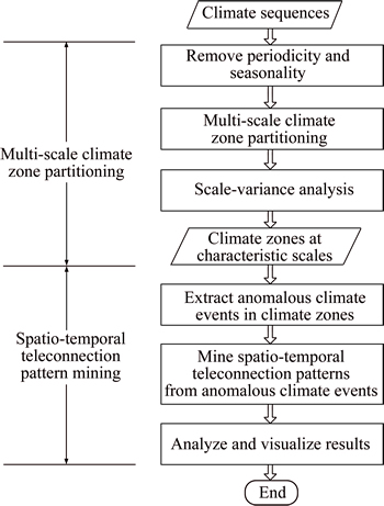
Fig. 1 Spatio-temporal teleconnection pattern mining framework

3 Multi-scale climate zone partitioning

3.1 Removal of temporal autocorrelation

Removal of temporal autocorrelation, e.g., periodicity and seasonality, in climate sequences caused by solar radiance is the key issue before extracting anomalous climate events [2, 7, 9, 24]. In this study, the monthly Z-core is used to remove the temporal autocorrelation due to its relatively high efficiency and simplicity, represented as

                                  (1)

where x_i is the attribute value in a specific month; denotes the average attribute value in the same month with x_i corresponding to all years in the entire time series; σ is the corresponding standard deviation. Figure 2(a) shows an original time series of sea surface temperature for one spatial region while the time series in Fig. 2(b) is obtained by using the Monthly Z-score method. The abscissa represents the 348 months from 1982 to 2010 according to the time order, i.e., January 1982, February 1982, …, and December 2010. Comparing Fig. 2(b) with Fig. 2(a), one can see that periodicity and seasonality of the temperature disappear.

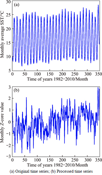
Fig. 2 Removal of temporal autocorrelation in climate time series:

Further, quantile–quantile plot is performed to investigate the distribution of the transformed time series, and scatter diagrams are used to explore the relationship between two transformed time series A and B. It is found that the distribution of transformed time series can be regarded as approximately normal distribution, and the relation ship between two transformed time series can be regarded as being approximately linear. Some results of the analyses are shown in Fig. 3. On this basis, the Pearson correlation coefficient can be considered an indicator to measure the similarity between transformed time series [8, 36]. Given two climate time series with the periodicity and seasonality removed, the Pearson correlation coefficient between them is utilized to measure their similarity. It can be expressed as

          (2)

In Eq. (2), d is the length of time series; x_k and y_k denote the values of the kth value of the processed time series X and Y, respectively; and denote the average values of the processed time series X and Y,respectively; R(X, Y) takes a value between –1 and 1. The closer this value is to 1, the more similar the X and Y are; the closer it is to –1, the more dissimilar the X and Y are.

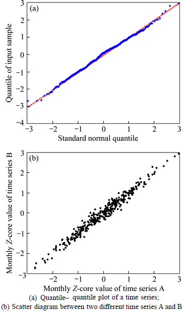
Fig. 3 Quantile–quantile plot and scatter diagram for monthly Z-core of sea surface temperature time series:

3.2 Multi-scale climate zones partitioning

To handle the effect of spatial scale on climate zone partitioning, a modified scale-space regionalization method is developed to obtain multi-scale climate zones.

For each climate sequence X, Y is one of the spatially neighbors of X, denoted as SN(X), and satisfies that. If then the gradient direction between X and Y with X as center is defined as X→Y; otherwise, the gradient direction is defined as Y→X. Further, if there is no climate sequence in SN(X) whose gradient direction points to X, then X is identified as a local minima. Similarly, if the gradient directions of climate time series in SN(X) all point to X, then X is identified as a local maxima.

The clustering process starts from a local minima, and is guided by the gradient direction until a local maxima is reached. All the climate sequences between local minima and local maxima form a cluster. Figure 4 gives an example to illustrate the scale-space clustering process. Regions 1, 6, and 8 are local maxima, regions 3 and 4 are local minima, and regions 2 and 5 are neither. One can see that two transfer directions can be selected for region 4. To ensure that there is just one transfer direction at each time, one of them has to be deleted. If region 7 is chosen as the center, region 4 has the most similar value with region 7. However, if we choose region 4 as the center, region 5 is the most similar with region 4. Therefore, the transfer direction between regions 4 and 7 was deleted. Based on this updated transfer direction, regions 1, 2, and 3 will be clustered into zone I and the average value of regions 1, 2 and 3 acts as the new value for zone I. Similarly, regions 4, 5, and 6 will be clustered into zone II, and zone III will be obtained by merging regions 7 and 8. The new zones, I, II and III, are the partitioning results obtained at spatial scale 1. Zones I, II, and III will be used as regions to cluster at the next spatial scale. The iteration will end when all regions are merged into one big zone.

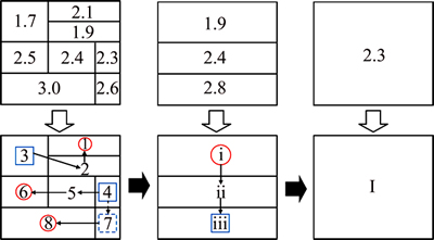
Fig. 4 An example of multi-scale regionalization

3.3 Scale-variance analysis

There is necessity to further select an optimal partitioning result from the obtained climate zones at different spatial scales. In this study, scale-variance analysis method developed for identifying spatial hierarchy and characteristic scale in geography is used to identify the optimal partitioning result [34]. The partitioning result at the characteristic scale identified by the scale variance analysis method will be further used. The statistical model of scale variance analysis can be described as

           (3)

where is the attribute value of a climate zone at the finest scale (the climate zones at the finest scale is just the initial dataset); μ is the grand mean attribute value of all climate zones at the finest scale and other items are the scale variance components that represent the effect of those climate zones at corresponding scales. The scale variance component can be obtained by computing the sum of squares and partitioned sums of squares at each scale. The readers of interest may refer to [34] for details. When the values of scale variance components are plotted against scale, the scale corresponding to local peak in scale variance is identified as characteristic scale. The climate zones obtained at characteristic scale imply that there is highly variability of spatial heterogeneity at that scale, which is an indication of the main characteristics of geography phenomenon [30]. Therefore, the climate zones obtained at characteristic scale are more suitable for further analysis.

4 Spatio-temporal teleconnection pattern mining

To mine spatio-temporal teleconnection patterns among the obtained climate zones, abnormal climate events (or climate event sequences) are extracted from each climate zone. Then, the mining process performed based on the concept of sliding time windows [14] is introduced. An analysis is subsequently made to verify the results, and visualization is provided.

1) Climate events and anomalous climate events: Given a climate sequence CS_i, each time stamp combined with its recorded climate attribute value is defined as a climate event. By handling all climate attribute values in CS_i with descending sort, those time stamps recording the largest 10% or the smallest 10% of the attribute values are defined as anomalous climate events (e.g., abnormally high and low temperature events), denoted as ACE(c_attr_i, t_j).

2) Sliding time windows: For a climate sequence CS_i, a sliding time window can be defined as where st_l is the start time, et_l is the end time of , and width is the width taking equals as et_l–st_l+1. The width of each window is preset as the same. To ensure that each event appears in the sliding time windows with the same frequency, the first window contains only the first event and the last window contains only the last event. In this case, the number of windows is T_e–T_s+width–1, where T_s and T_e are the start and end time of CS_i, respectively. In Fig. 5, an example is utilized to illustrate the setting of sliding time windows. The width of sliding time windows is set to 3. Three kinds of windows, which are represented by dashed boxes, can be obtained, where their lengths are 1(STW_1→1 and STW_17→17), 2(STW_1→2 and STW_16→17) and 3 (STW_6→8), respectively.

3) Spatio-temporal teleconnection patterns: Two climate sequences, CS_i and CS_j , describing two climate zones with different climate attributes, can be respectively divided into a set of sliding time windows based on a given window width. With the guide of earth scientists, anomalous event of one climate attribute is considered the antecedence while anomalous event of the other climate attribute is the consequence. A spatio- temporal teleconnection pattern STTP is a process in which the consequence occurs after the antecedence appearing in the same sliding time window, which can be represented as

For example, in a sliding time window with a width of 6 months, the observation, “the sea surface temperature of a climate zone marked as A is anomalously highand the land precipitation of a climate zone marked as B is anomalously high”, is a spatio-temporal teleconnection pattern.

4) The significance degree: Given a STTP_k, the number of sliding time windows with the occurrence of antecedence and the number of sliding time windows with the occurrence of STTP_k are denoted as |STTP_k_A| and |STTP_k|, respectively. The significance degree of STTP_k can be expressed as

                     (4)

If SD(STTP_k) is larger than a given threshold MIN_SD, then STTP_k is considered to be significant.

5 Experimental results

In this study, the proposed framework is performed on the climate data products to mine spatio-temporal teleconnection patterns between anomalous sea and land climate events. Sea climate data include: 1) the global sea surface temperature obtained from the optimum interpolation sea-surface temperature V2.0 provided by the National Oceanic and Atmospheric Administration (NOAA); and 2) the global monthly sea level pressure obtained from the NCEP reanalysis derived data provided by the NOAA. Land climate data include:1) the global land precipitation obtained from the full data product provided by the Global Precipitation Climatology Centre (GPCC); and 2) the land temperature of China obtained from the China Meteorological Administration.

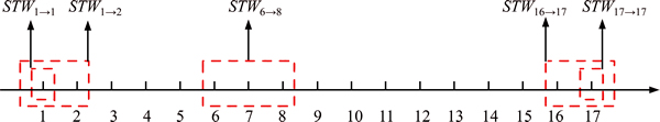
Fig. 5 Illustration of sliding time windows

The sea and land climate sequences are in the form of grid networks partitioned by latitude and longitude with the spatial resolutions of 1°×1° (sea surface temperature, land precipitation and land temperature) and 2.5°×2.5° (sea level pressure), recording time series with quantitative attribute values with the time resolution of one month. In addition, the time range of sea surface temperature and land precipitation is from January 1982 to December 2010, while the period of January 1982 to December 2004 is selected with respect to sea level pressure and land temperature.

5.1 Case study 1: mining of spatio-temporal teleconnection patterns between anomalous sea surface temperature and land precipitation

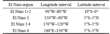
Currently, there is some prior knowledge about the teleconnection patterns between anomalous sea surface temperature, e.g., El Nino and La Nina, and land precipitation. Four El Nino regions shown in Table 1, i.e., El Nino 1+2, El Nino 3, El Nino 3.4 and El Nino 4 can be used to define the climate indices that indicate the El Nino and La Nina phenomena [7]. The anomalously high sea surface temperature of El Nino regions refers to the El Nino event. Then, the rainfall of Peru, Ecuador, and Chile will be anomalously high and droughts will occur in the northeast of Brazil, Southeast Asia, parts of Australia, and the southeast of Africa. When the sea surface temperature of El Nino regions is anomalously high, La Nina events occur. Then, Indonesia, the Philippines, and Australia will receive abundant rainfall, while droughts will occur in the middle of Argentina and the south of Brazil. These prior knowledge can be considered benchmark to evaluate the performance of the proposed framework in this study.

Table 1 Spatial scope of four El Nino regions

The modified multi-scale regionalization method was first utilized to obtain multi-scale climate zones of sea surface temperature and land precipitation. Then, scale-variance analysis was performed to identify the climate zones at characteristic scale, and the scale variance of multi-scale climate zones is shown in Fig. 6. By identifying local peak in scale variance, scale 6 was determined as the characteristic scale of sea surface temperature zones and scale 7 was determined as the characteristic scale of land precipitation zones. Further, a correlation coefficient analysis was performed to compare the sea surface temperature of each zone with those of four known El Nino regions. Those zones having the maximum correlation coefficient with the four known El Nino regions were correspondingly marked as the identified four El Nino regions, and the correlation coefficients were all larger than 0.96. In addition, more than 90% grids in the known El Nino regions again appeared in the identified ones. This fact to a large degree also indicates that the obtained climate zones are effective.

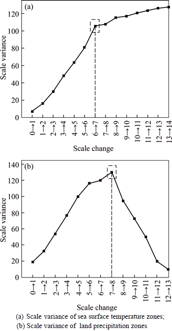
Fig. 6 Scale variance of multi-scale climate zones discovered from sea surface temperature and land precipitation:

To mine teleconnection patterns between the four identified El Nino regions and the obtained land precipitation zones, the width of sliding time windows and MIN_SD should be set by users. Through the analysis of related researches, there were no specific criterions that guide the selection of these two parameters and so amounts of experiments were implemented to explore the association patterns from different combinations of parameters [1, 11, 18, 24]. In light of this, this study set the widths of the sliding windows as 3, 6, and 9 months to explore the effect of abnormal events in sea climate zones on the land climate zones on the scale of seasonality in a year. And the MIN_SD was set to vary from 0.4 to 1 with the interval of 0.05 to extract those significant teleconnection patterns in which antecedence and consequence included sea and land climate zones covering relatively larger regions of the earth. The spatio-temporal teleconnection patters related with El Nino regions can be respectively described as follows.

(I) The sea surface temperature of El Nino regions is anomalously high => The land precipitation of western coast of South America, south Brazil, south USA, west Europe, east Africa, middle and lower Yangtze River in China will be anomalously strong.

(II) The sea surface temperature of El Nino regions is anomalously high => The land precipitation of northeast Brazil, middle America, south Africa, east Australia will be anomalously weak.

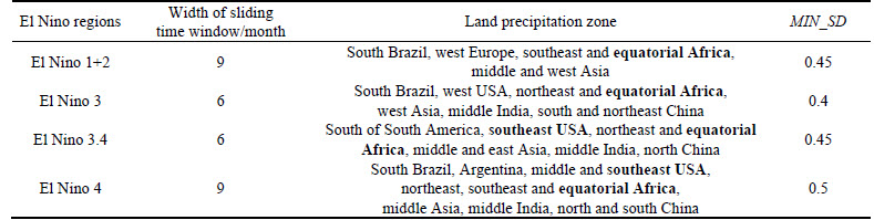
(III) The sea surface temperature of El Nino regions is anomalously low => The land precipitation of northeast Brazil, south Africa, India will be anomalously strong.

(IV) The sea surface temperature of El Nino regions is anomalously low => The land precipitation of southeast USA, equatorial regions in Africa will be anomalously weak.

The discovered four teleconnection patterns between El Nino regions and land precipitation zones are summarized in Tables 2–5.

Table 2 Discovered pattern (I) between El Nino regions and land precipitation zones

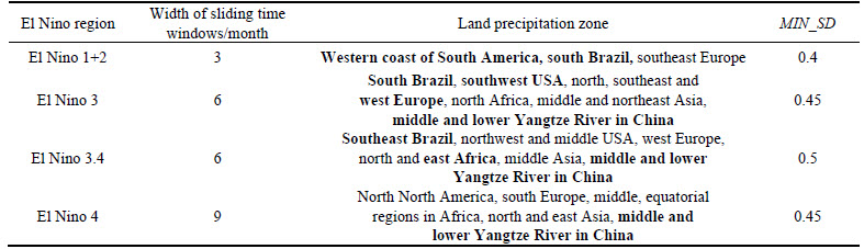
Table 3 Discovered pattern (II) between El Nino regions and land precipitation zones

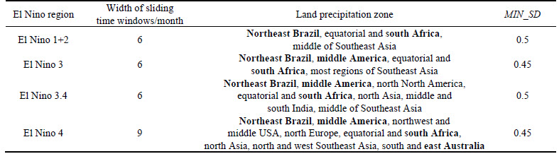
Table 4 Discovered pattern (III) between El Nino regions and land precipitation zones

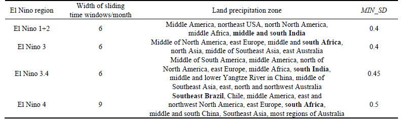
Table 5 Discovered pattern (IV) between El Nino regions and land precipitation zones

Indeed, the effectiveness of the proposed framework can be verified by using the prior knowledge of El Nino and La Nina phenomena. In addition, some unknown patterns are also discovered, which can be summarized as follows.

(I) The sea surface temperature of some sea zones is anomalously high => The land precipitation of some land zones will be anomalously high.

(II) The sea surface temperature of some sea zones is anomalously high => The land precipitation of some land zones will be anomalously low.

(III) The sea surface temperature of some sea zones is anomalously low => The land precipitation of some land zones will be anomalously high.

(IV) The sea surface temperature of some sea zones is anomalously low => The land precipitation of some land zones will be anomalously low.

Table 6 describes these unknown teleconnection patterns in detail. These teleconnection patterns may be further used to define new climate indices, and it is also demonstrated that the proposed framework is feasible to explore unknown patterns from climate sequences.

5.2 Case study 2: mining of spatio-temporal teleconnection patterns between anomalous sea level pressure and land temperature

To discover teleconnection patterns between anomalous sea level pressure and land temperature, the multi-scale climate zones are first obtained, and their scale variance is shown in Fig. 7. By identifying local peak in scale variance, scale 4 is determined as the characteristic scale of sea level pressure zones and scale 5 is determined as the characteristic scale of land temperature zones.

Being similar with case study 1, the widths of the sliding time windows were respectively preset at 3, 6, and 9 months, and the MIN_SD varied from 0.4 to 1 with the interval of 0.05. The four kinds of teleconnection patterns discovered are described as follows.

(I) The sea level pressure of some sea zones is anomalously high => The land temperature of some land zones will be anomalously high.

(II) The sea level pressure of some sea zones is anomalously high => The land temperature of some land zones will be anomalously low.

(III) The sea level pressure of some sea zones is anomalously low => The land temperature of some land zones will be anomalously high.

(IV) The sea level pressure of some sea zones is anomalously low => The land temperature of some land zones will be anomalously low.

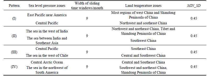
Due to constraints on the size of this article, only some teleconnection patterns whose antecedence and consequence include relatively large sea and land climate zones are described in Table 7. Here for example, when the sea level pressure of the south Indian Ocean around Southeast Asia is anomalously high, it is very likely that the land temperature of the southwestern regions of China will be anomalously high within 9 months. These patterns are all unknown and can be further analyzed in more detail to discover the relationship between sea and land climate. Moreover, these patterns also can be converted into meaningful knowledge to assist decision-making.

6 Conclusions

A framework for mining spatio-temporal teleconnection patterns of anomalous climate events between sea and land was proposed based on multi-scale regionalization. First, a modified scale-space regionalization method is developed to detect multi-scale climate zones, and scale variance analysis method is employed to identify the climate zones at characteristic scales. It is illustrated that the effect of both positive spatial autocorrelation and spatial scale on mining teleconnection patterns can be handled. Then a time association rules mining method based on sliding time windows is further utilized to mine teleconnection patterns between sea and land climate zones. To assess the validity of the proposed framework, the known climate indices (e.g., the El Nino index) and teleconnection patterns between anomalous sea surface temperature and land precipitation are used as the benchmarks. The experiments illustrate that the proposed framework can precisely identify the known climate indices and discover the known teleconnection patterns. Compared with existing method, the subjectivity in the discovery of teleconnection patterns is significantly reduced. In addition, some previously unknown teleconnection patterns also can be discovered, which can be further used for the prediction of land climate.

Table 6 Unknown patterns between anomalous sea surface temperature and land precipitation

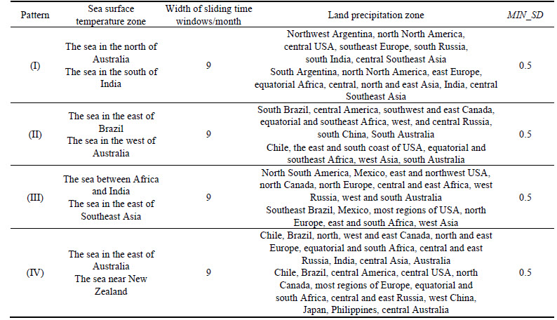
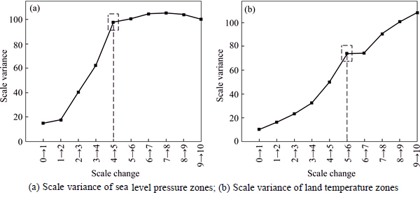
Fig. 7 Scale variance of multi-scale climate zones discovered from sea level pressure and land temperature:

Table 7 Unknown patterns between anomalous sea level pressure and land temperature

It should be pointed out that the proposed framework has similar limitations with existing methods, that is, the discovered teleconnection patterns depend on the width of sliding time windows and the threshold MIN_SD. Indeed, the determination of optimal parameters for discovery of teleconnection patterns should be further investigated. It would be worthwhile to determine these parameters by incorporating domain knowledge. In addition, with respect to more than two parameters, the multiple parameters based climate zone regionalization and the cascading relationships involving these parameters should be further explored and embedded in the process of unveiling spatio-temporal teleconnection patterns. Considering the time dimension, the dynamic of teleconnection patterns should also be further investigated in our future work.

References

[1] XUE Cun-jin, DONG Qing, FAN Xing. Spatiotemporal association patterns of multiple parameters in the northwestern Pacific Ocean and their relationships with ENSO [J]. International Journal of Remote Sensing, 2014,35(11, 12): 4467–4483.

[2] TAN P, STEINBACH M, KUMAR, V. Finding spatio-temporal patterns in earth science data [C] // KDD Workshop on Temporal Data Mining. San Francisco, USA: KWTDM, 2001.

[3] WOLD S. Principal component analysis [J]. Chemometrics and Intelligent Laboratory Systems, 1987, 2(1–3): 37–52.

[4] KLEMA V, LAUB A. The singular value decomposition: Its computation and some applications [J]. IEEE Transactions on Automatic Control, 1980, 25(2): 164–176.

[5] GOZOLCHIANI A, YAMASAKI K, GAZIT O, HAVLIN S. Pattern of climate network blinking links follows El Nino events [J]. Europhysics Letters, 2008, 83(2): 28005.

[6] DONGES J F, ZOU Yong, MARWAN N, KURTHS J. Complex networks in climate dynamics [J]. The European Physical Journal Special Topics, 2009, 174(1): 157–179.

[7] STEINBACH M, KLOOSTER S, POTTER C. Discovery of climate indices using clustering [C]// ACM SIGKDD International Conference on Knowledge Discovery and Data Mining. Washington DC, USA: ACM, 2003: 446–455.

[8] STORCH H, ZWIERS F. Statistical analysis in climate research [M]. London: Cambridge University Press, 1999.

[9] STEINBACH M, TAN P, KUMAR V. 2002. Temporal data mining for the discovery and analysis of ocean climate indices [C] // KDD Workshop on Temporal Data Mining. Edmonton, Canada: KWTDM, 2002: 1–12.

[10] TADESEE T, WILHITE D A, HARMS S K, HAYES M J, GODDARD S. Drought monitoring using data mining techniques: a case study for Nebraska, USA [J]. Natural Hazards, 2004, 33(1): 137–159.

[11] WU Tian-shu, SONG Guo-jie, MA Xiu-jun, XIE Kun-qing, GAO Xiao-ping, JIN Xing-xing. Mining geographic episode association patterns of abnormal events in global earth science data [J]. Science in China Series E: Technological Sciences, 2008, 51(1): 155–164.

[12] DARK S, BRAM D. The modifiable areal unit problem (MAUP) in physical geography [J]. Progress in Physical Geography, 2007, 31(5): 471–479.

[13] HAY G, MARCEAU D, DUBE P, BOUCHARD A. A multiscale framework for landscape analysis: Object-specific analysis and upscaling [J]. Landscape Ecology, 2001, 16(6): 471–490.

[14] MANNILA H, TOIVONEN H, VERKANMO A. Discovery of frequent episodes in event sequences [J]. Data Mining and Knowledge Discovery, 1997, 1(3): 259–289.

[15] DAS G, LIN K I, MANNILA H. Rule discovery from time series [C]// International Conference on Knowledge Discovery and Data Mining. New York, USA: AAAI, 1998: 16–22.

[16] HARMS S K, DEOGUN J, TADESSE T. Discovering sequential association rules with constrains and time lags in multiple sequences [C]// International Symposium on Methodologies for Intelligent Systems. Lyon, France: Springer, 2002: 432–441.

[17] XUE Cun-jin, LIAO Xiao-han. Novel algorithm for mining ENSO- oriented marine spatial association patterns from raster-formatted datasets [J]. International Journal of Geo-Information, 2017, 6(5): 139.

[18] XUE Cun-jin, FAN Xing, DONG Qing, LIU Jing-yi. Using remote sensing products to identify marine association patterns in factors relating to ENSO in the pacific ocean [J]. International Journal of Geo-Information, 2017, 6(1): 32.

[19] TAN P, STEINBACH M, KUMAR, V. Introduction to data mining [M]. Boston, USA: Addison Wesley Press, 2006.

[20] FOVELL R, FOVELL M. Climate zones of the conterminous United States defined using cluster analysis [J]. Journal of Climate, 1993, 6(11): 2103–2135.

[21] DEGAETANO T. Spatial grouping of United States climate stations using a hybrid clustering approach [J]. International Journal of Climatology, 2001, 21(7): 791–807.

[22] STEINHAEUSER K, CHAWLA N V, GANGULY A R. An exploration of climate data using complex networks [J]. Acm Sigkdd Explorations Newsletter, 2010, 12(1): 25–32.

[23] STEINHAEUSER K, CHAWLA N V. Identifying and evaluating community structure in complex networks [J]. Pattern Recognition Letters, 2010, 31(5): 413–421.

[24] XUE Cun-jin, SONG Wan-jiao, QIN Li-juan, DONG Qing, WEN Xiao-yang. A spatiotemporal mining framework for abnormal association patterns in marine environments with a time series of remote sensing images [J]. International Journal of Applied Earth Observation and Geoinformation, 2015, 38: 105–114.

[25] KAWALE J, STEINBACH M, KUMAR V. Discovering dynamic dipoles in climate data [C]// SIAM Conference on Data Mining. Mesa, USA: SIAM, 2011: 107–118.

[26] XUE Cun-jin, SONG Wan-jiao, QIN Li-juan, DONG Qing, WEN Xiao-yang. A mutual-information-based mining method for marine abnormal association rules [J]. Computers & Geosciences, 2015, 76: 121–129.

[27] XUE Cun-jin, DONG Qing, LI Xiao-hong, FAN Xing, LI Yi-long, WU Shu-chao. A remote-sensing-driven system for mining marine spatiotemporal association patterns [J]. Remote Sensing, 2015, 7(7): 9149–9165.

[28] OPENSHAW S. A geographical solution to scale and aggregation problems in region-building, partitioning and spatial modeling [J]. Transactions of the Institute of British Geographers, 1977, 2(4): 459–472.

[29] WU Jian-guo. Hierachy and scaling: extrapolating information along a scaling ladder [J]. Canadian Journal of Remote Sensing, 1999, 25(4): 367–380.

[30] ZHANG Na, ZHANG Hong-yan. Scale variance analysis coupled with Moran’s I scalogram to identify hierarchy and characteristic scale [J]. International Journal of Geographical Information Science, 2011, 25(9): 1525–1543.

[31] LEUNG Y, ZHANG Jiang-she, XU Zong-ben. Clustering by scale- space filtering [J]. IEEE Transactions on Pattern Analysis and Machine Intelligence, 2002, 22(12): 1396–1410.

[32] LUO Jian-cheng, ZHOU Cheng-hu, LEUNG Y, ZHANG Jiang-she, HUANG Ye-fang. Scale-space theory based regionalization for spatial cells [J]. Acta Geographica Sinica, 2002, 57(2): 167–173.

[33] MU Lan, WANG Fa-hui. A scale-space clustering method: mitigating the effect of scale in the analysis of zone-based data [J]. Annals of the Association of American Geographers, 2008, 98(1): 85–101.

[34] MOELLERING H, TOBLER W. Geographical variances [J]. Geographical Analysis, 1972, 4(1): 34–50.

[35] IPCC. Climate change 2001: the science of climate change [R]. London: Contribution of Working Group I to the Third Assessment Report of the Intergovernmental Panel on Climate Change, 2001.

[36] HAUKE J, KOSSOWSKI T. Comparison of values of Pearson’s and Spearman’s correlation coefficients on the same sets of data [J]. Quaestiones Geographicae, 2011, 30(2): 87–93.

(Edited by YANG Hua)

Cite this article as: XU Feng, SHI Yan, DENG Min, GONG Jian-ya, LIU Qi-liang, JIN Rui. Multi-scale regionalization based mining of spatio-temporal teleconnection patterns between anomalous sea and land climate events [J]. Journal of Central South University, 2017, 24(10): 2438–2448. DOI:https://doi.org/10.1007/s11771-017-3655-x.

Foundation item: Projects(41601424, 41171351) supported by the National Natural Science Foundation of China; Project(2012CB719906) supported by the National Basic Research Program of China (973 Program); Project(14JJ1007) supported by the Hunan Natural Science Fund for Distinguished Young Scholars, China; Project(2017M610486) supported by the China Postdoctoral Science Foundation; Projects(2017YFB0503700, 2017YFB0503601) supported by the National Key Research and Development Foundation of China

Received date: 2017-04-12; Accepted date: 2017-09-28

Corresponding author: SHI Yan, Assistant Professor, PhD; Tel: +86–18615582266; E-mail: whu_shiy@126.com