J. Cent. South Univ. (2016) 23: 1944-1953

DOI: 10.1007/s11771-016-3251-5

Line of sight waypoint guidance for a container ship based on frequency domain identification of Nomoto model of vessel

M. T. Ghorbani

Instituto Superior Técnico, Torre Norte-8.17, 1049-001 Lisboa, Portugal

Central South University Press and Springer-Verlag Berlin Heidelberg 2016

Abstract: CIFER software is used to identify steering and roll dynamics of a container ship. In this software, advanced features such as the Chirp-Z transform (CZT) and composite window optimization are applied to the time history of steering and roll dynamics to extract high quality frequency responses. From the extracted frequency responses, two linear transfer functions of Nomoto model are fitted for yaw and roll dynamics of the vessel. Based on the identified Nomoto model, a PID heading controller and a Kalman filter observer are constructed. The simulation results of heading controller for line of sight (LOS) waypoint guidance show excellent tracking of pilot inputs in the presence of wave induced motions and forces.

Key words: container ship; Nomoto model; Kalman filter; frequency domain identification; CIFER software

1 Introduction

Systems for waypoint guidance are used for ships. These systems consist of a waypoint generator with human interface. The selected waypoints are stored in a database and used for generation of a trajectory or a path for the moving vessel to follow.

LOS guidance is considered a very advanced methodology for marine steering systems. A line of sight vector from the vessel to the next waypoint or a point on the path between two waypoints can be computed for heading control. If the vessel is equipped with a course autopilot the angle between the line of sight vector and the pre-described path can be used as set point for the course autopilot. This will force the vessel to track the path.

The other part of a vessel steering system is heading controller. The majority of controllers are model based controllers. This type of controllers can be constructed based on the mathematical model of the vessel. The ideal for steering system is that the vessel mathematical model can predict the behavior of the model as fast and accurately as possible. This can be done by constructing a very accurate linear model for the vessel dynamics.

On the other hand, system identification is the process of knowing the structure of the mathematical model of a system from the measurements of its inputs and outputs. Identification methods generally trade simplicity of experiments for computational efficiency [1]. They also offer an alternative way of determining ship steering dynamics directly by recording how a ship reacts to changes in the rudder angle. The input signal to the ship dynamics (here, is the rudder angle) must be, in a frequency sense, rich enough to excite all modes of interest of the vessel. A good input signal with mentioned features can be a frequency sweep.

Some of the established system identification methods in this area are recursive maximum likelihood estimation [1], indirect model reference adaptive method [2], recursive least square estimation method [2], neural networks method [3], support vector regression method [4] and the spectral analysis method [5].

In the present paper a comprehensive spectral analysis is performed to determine the steering dynamics of a container ship. Two key features of the spectral analysis described herein, and implemented in CIFER software package, are CZT and composite windowing optimization [6]. These features produce a frequency- response database of exceptionally high accuracy and resolution over a broad dynamic range for real test data. An important byproduct of this analysis is the coherence function, which provides key information about the frequency-response accuracy and the degree of model linearity.

Transfer-function modelling of steering dynamics is next step in the system identification procedure. In this article a first order Nomoto model [7] is chosen and its constants are identified by the proposed method. The identification process of the current paper is done in CIFER software.

CIFER is a tool to solve the aircraft system identification problem based on the frequency response approach. The Army/NASA Rotorcraft Division at Ames Research Center in United States jointly developed it in 80’s. Mainly, this software is composed of six core programs that carry out the basic computations of the frequency response identification method. They are FRESPID, MISOSA, COMPOSITE, NAVFIT, DERIVID, and VERIFY [7]. The six core programs within the CIFER perform the following processes: data conditioning and performing CZT, FRESPID; multi- input conditioning, MISOSA; window combination, COMPOSITE; transfer-function model identification, NAVFIT; state-space model identification, DERIVID and model verification, VERIFY. In the current paper, only FRESPID and NAVFIT are used to extract the transfer function of heading dynamics. More details of the programs used in this paper can be found in section 3.

After completion of the identification process, the PID controller gains in terms of the Nomoto constants are calculated and a reference model will be added to the controller in order to achieve more accurate and rapid course-changing manoeuvres. The final step is to design a Kalman filter based on identified Nomoto model coefficients. To verify the performance of the designed PID controller and Kalman observer, a line of sight waypoint guidance scenario in the wave field is proposed. Results show excellent performance of the controller and observer even in the serve conditions of sea waves.

Recent articles in the field of guidance of marine vessels are largely based on the nonlinear dynamics of marine vehicles [8-12]. Such works have been used very tedious calculation of nonlinear controller which makes the implementation of such algorithms very hard. The key feature of the current paper is that the designed controller is based on linear model of the vessel which has a very good performance in waypoint control even in the presence of sea loads.

After a brief introduction, the remainder of this paper is organized as follows: in Section 2, the 4-DOF vessel model is presented. In Section 3, the frequency domain identification process is addressed to model steering dynamics of the vessel based on the Nomoto model. The simulation results of the LOS waypoint guidance PID controller and Kalman filter estimation are presented in Section 4 together with some discussions on the design process, followed by the conclusions in Section 5.

2 Description of container ship model

The mathematical model presented here consists of a nonlinear manoeuvring model. Note that in order to have high quality identification, it is necessary to test models in calm water to decrease noise-to-signal ratio [6]. So, the effect of sea waves on the vessel dynamics is neglected in this study, i.e. seakeeping, during the identification process.

A mathematical model for a single-screw high- speed container ship (often referred to as S175 in the marine engineering community) in surge, sway, roll and yaw has been presented in Ref. [13]. This 4-DoF dynamical ship model is highly nonlinear with 10 states: x=[u, v, r, x, y, ψ, p, f, n, δ]^T and 2 control inputs: u=[u_c, δ_c]^T where u, v, r and p are the surge velocity, sway velocity, yaw rate and roll rate with respect to the ship-fixed frame, respectively; the corresponding displacements with respect to the inertial frame are denoted by x, y. ψ and f are the yaw and roll Euler angles, respectively. Other two states are the propeller shaft speed n and the rudder angle δ. The inputs to the model are the commanded propeller speed n_c and commanded rudder angle δ_c, respectively. The actuator input saturation and rate limits are also incorporated in this model so that |δ|≤45° and 20 (°)/s and 0T and inputs of the vessel according the following equation:

      (1)

where and L is the ship length.

The nonlinear equations of motion in 4-DoF are given by

       (2)

where m' denotes the ship mass; m'_x and m'_y denote the added mass in the x and y directions, respectively; I'_x and I'_z denote the moment of inertia and J'_x and J'_z denote the added moment of inertia about the x and z axes, respectively. Furthermore,denotes the x-coordinate of the center of m'_y. l'_x and l'_y are the z-coordinates of the centers of m'_x and m'_y, respectively. W' is the ship displacement; GM' is the metacentric height and x'_G is the location of the center of gravity in the x-axis. All the primes mean the corresponding dimensionless terms. Please see Appendix E.1.3 in Ref. [13] for the details.

The values for hydrodynamic forces X', Y' and moments K', N' in Eq. (2) are given in the Appendix E.1.3 of Ref. [13].

Also, the dynamics of the rudder and propeller are incorporated by

                             (3)

where T_δ and n_δ are time constants.

The motion equations can be transformed into the control-oriented dynamics equations as follows:

 (4)

where m'₁₁=m'+m'_x; m'₂₂=m'+m'_y; m'₃₂=-m'_yl'_y; m'₄₂=-m'_yα'_y; m'₃₃=I'_x+J'_x; m'₄₄=I'_z+J'_z and detM'= m'₂₂m'₃₃m'₄₄-m'²₃₂ m'₄₄-m'²₄₂ m'₃₂.

In the current paper, for the sake of simplicity, it is assumed that the propeller shaft speed n is to be constant value of 60 r/min. Regarding this assumption, there will be only one input to the nonlinear model of the vessel, namely the commanded rudder angle δ_c.

In summary, the control input to the nonlinear manoeuvring model of the vessel is the commanded rudder angle. The output of the model that needs to be controlled is the yaw angle. The control strategy determines rudder angle for heading control, while considering the roll angle of the vessel not to exceed a certain value.

3 Frequency-domain system identification procedure

The steps required for the frequency-domain system identification procedure includes: 1) the collection of time-domain data from the excitation of the test bench with frequency sweep inputs, 2) data processing, 3) spectral analysis and identification of frequency response functions (non-parametric system identification), 4) transfer function modelling (parametric identification). The step 3 and step 4 are done with FRESPID and NAVFIT modules of CIFER software, respectively.

3.1 Time-domain data collection and data processing

The first step in the system identification process is the collection of a well-suited time-history database. Since the only control input in the identification process is the commanded rudder angle, it is constructed as a frequency-sweep, using the following equation [14]:

      (5)

where A is the sweep amplitude and T_rec is the total sweep record length. The values C₁=4.0 and C₂=0.0187 have been found to be suitable for a wide range of applications.

Experience for a wide range of applications has shown that the total sweep record length ω_min should be as follows [7]:

                                 (6)

Note that the record starts and ends with zero rudder angle to ensure a good steady-state condition.

To enrich the spectral content, a band-limited white- noise component is also added to the sweep:

                    (7)

A typical rms (lσ) level of the noise signals is selected as

                           (8)

The white-noise component should be processed with a low-pass filter (ω_f=ω_max) to suppress high- frequency content in the excitation.

Figure 1 shows the constructed rudder frequency sweep for 100 s. The sweep amplitude, A, is 45°, ω_min is 1 π/10 s, and ω_max is 8 rad/s. As seen in this figure, to ensure a steady-state condition at the beginning and at the end, the signal is set to zero for 3 s. The constructed rudder frequency sweep is then applied to the ship model to collect the roll and yaw angle of the vessel. The next step in identification procedure is spectral analysis of collected yaw and roll data.

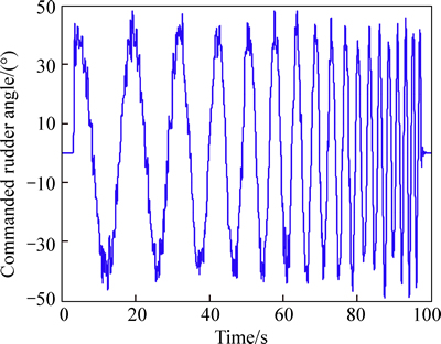
Fig. 1 Commanded rudder frequency sweep input

3.2 Spectral analysis

The frequency response for each input-output pair is computed using CZT. CZT is a highly flexible fast Fourier transform (FFT) algorithm that has several advantages over the standard discrete Fourier transform DFT [11].

The accuracy of the low and high frequency ends of the frequency responses is improved through overlapped windowing technique [7, 15]. At the same time, the coherence function for each frequency response is calculated. If the system was perfectly linear and the estimated spectral densities were noise-free, a coherence value of 1 would result. In general, a coherence value greater than 0.6 is considered satisfactory (see Refs. [7] and [13] for more details).

3.3 Transfer function modelling

Direct transfer function fitting of the frequency response functions is a straight, simple and useful way of parameterizing the system dynamics. A numerical optimization algorithm determines the set of unknown quantities (gain, pole and zero locations and phase lag) that minimizes the magnitude and phase errors between the desired SISO transfer-function model and the associated composite frequency response estimate [16]. An appropriate transfer-function model for the vessel steering dynamics is Nomoto’s first order model. NAVFIT module of CIFER software handles the optimization process to determine the Nomoto model coefficients.

The frequency range of the fit must be restricted to the frequency range over which the coherence function is satisfactory (greater than 0.6).

3.4 Results of identification process

In this section, the frequency-response identification concepts are demonstrated for the vessel. Two excitation signals are applied to the system for 100 s and 120 s sampled at 100 Hz. The time-history data from two separate trials for all outputs are then concatenated. The concatenated data record is segmented into 5 windows of length 44 s. An appropriate conditioning parameter is selected for the digital filter (ω_filter=5ω_max).

Since the higher-derivative measurements (angular rates) generally have better signal-to-noise content over a wider frequency range than do the attitude [7], the roll and yaw angular rate responses are identified and a 1/s correction is applied in the frequency domain to easily calculate the associated attitude responses. Figures 2 and 3 depict yaw and roll rate frequency responses, respectively. As it is shown, the vessel’s frequency response has coherence greater than 0.6 between frequency range of 0.2 rad/s to 4 rad/s. So, the vessel acts like a linear system in this frequency range.

Since the natural frequency of roll for the vessel is 0.93 rad/s [9], there is a peak about frequency of 1 rad/s in magnitude plot of roll rate in Fig. 3.

The identified transfer function model for yaw rate to commanded rudder angle within the frequency range of 0.4 to 4 is based on Nomoto’s first order model [1] as follows:

                                  (9)

where K=-0.075, T=4.5.

The frequency response of the identified transfer function model is seen in Fig. 4 to be identical to the simulated vessel data.

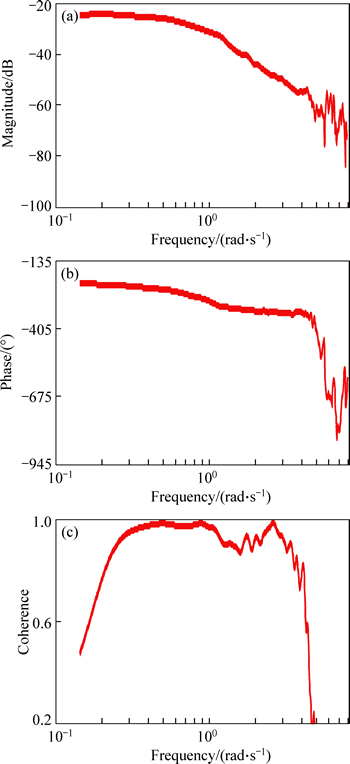
Fig. 2 Yaw rate frequency response

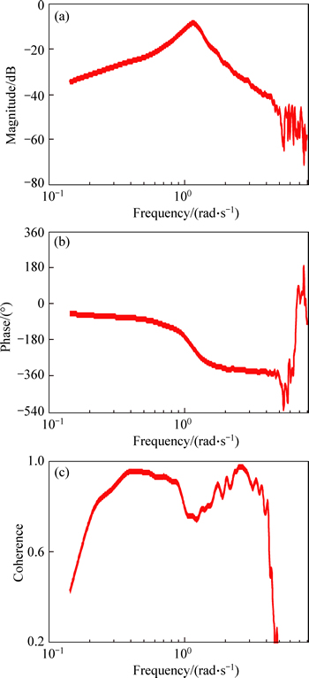
Fig. 3 Roll rate frequency response

The identified roll rate transfer function model is [13]:

                  (10)

where K₂=0.02, z₁=-16.55, ξ=0.1, ω_n=0.94, p₁=1.39.

Figure 5 shows roll rate frequency response of the identified transfer function model. As seen in this figure, the identified transfer function model for roll rate is very similar to the frequency response of the vessel roll rate.

4 Marine guidance, navigation and control systems

Figure 6 shows the logical structure of guidance,navigation and control systems and the data flow between the three subsystems. Diagram architecture and employed symbols are well-explained in the following sections. In the two following sections, wave inducted forces are neglected and the last section evaluates the performance of designed controller and observer considering effects of wave loads.

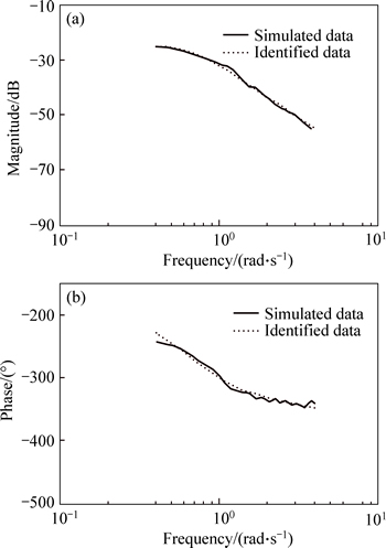
Fig. 4 Yaw rate simulated and identified frequency response

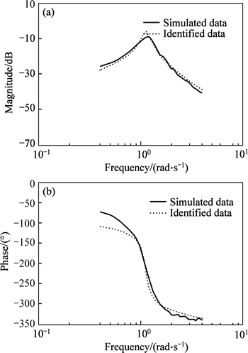
Fig. 5 Roll rate simulated and identified frequency response

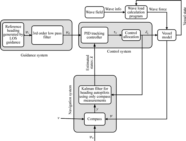
Fig. 6 Conceptual data flow diagram for generic GNC systems

4.1 PID heading controller

This section describes the design of the PID heading controller, based on the work done by MOREIRA et al [17]. Assuming that ψ is measured by using a compass, a PID controller will be presented as

      (11)

where τ_N is the controller yaw moment and K_p, T_d, T_i could be found by pole placement in terms of the natural frequency (ω_n) and relative damping ratio () of the first order system. The detailed information is presented in Refs. [13] and [17]. In the current case it is assumed that ω_n=1 rad/s and =1 as a critical damping. In Eq. (11), is the heading error. Here, ^ stands for the estimated state.

As seen in Fig. 6, there should be control allocation part in the control design procedure to compute the input command to the vessel model. For a rudder controlled craft, this is done by

A simple third-order filter for the purpose of course-keeping and turning capabilities is presented by

             (12)

where the reference ψ_r is the pilot heading input which can be determined through waypoint positions; _r is the relative damping ratio; and ω_n is the natural frequency.

4.2 Model for course autopilots observer design

In this section the model that is usually used to implement observers for autopilot wave filtering is discussed. As well, Kalman filter estimation is explained.

Here, the first-order, wave-induced motion is considered an output disturbance. Hence the measured yaw angle could be decomposed into

                               (13)

where ψ_w represents the first order wave-induced motion.

To estimate ψ and r and thus wave filtering, the state-space model that is used for Kalman filter design is introduced by

                          (14)

where x=[ξ_w, ψ_w, ψ, r, b]^T; u=τ_N;

where ω₀ and ξ_f are the wave filter parameters that represent the wave-induced yaw motion, b is the bias term, and are Gaussian white noises. The measurement equation is as follows:

                              (15)

where v represents zero-mean measurement Gaussian white noise introduced by the sensor. Also note that neither the yaw rate r nor the wave states ξ_w and ψ_w are measured in this process.

Finally, the state estimate propagation equation is:

                      (16)

where K is the Kalman gain matrix. For detailed information the reader is referred to Ref. [18].

The parameters of the first-order wave-induced motion model namely, ξ_f=0.1, ω₀=1.2 rad/s, and the standard deviation of the noise driving the filter are also assumed to be The standard deviation of the noise of the compass sensor is assumed to be 0.5°. Using the aforementioned data, a Kalman filter is designed.

Although, PID controller design and Kalman filtering are based on the identified model in calm water, it is more convenient to evaluate their performance in the wave field. Wave forces and moments are also added to the ship manoeuvring model (see Fig. 6). Details about the numerical test-bed were reported in Ref. [19]. Based on the this report, the beam sea where the angle between the vessel heading and dominant direction of the wave is 90°, has the largest yaw and roll moments. So, the ability of controller and observer is evaluated in this condition. In the following simulation, the ITTC spectrum is adopted with 1.25 m significant wave height (sea state 3), 1.2 rad/s peak frequency and default wave spreading factor 2 [20].

4.3 LOS guidance system

Let the vehicle mission be given by a set of way points. Hence we can define the LOS in terms of a desired heading angle. The desired route is most easily specified using waypoints (P₁, P₂, …, P_N) with coordinates P_i=(X_i, Y_i), i=1, …, N. The reference heading can then be obtained from the relationship:

                         (17)

where the current ship position (x, y) is calculated from kinematics equations. In a real system, GPS (global positioning system) can detect the position of the vessel.

The autopilot can hence be used in this way to move the ship toward waypoints. The switch between waypoints happens when the vessel lies within a circle of acceptance around the current waypoint. In the current work, the acceptance radius is 50 m.

Assuming that the vessel is located at the origin at the zero time and the 3 waypoint positions are (400, 800), (-400, 800) and (-600, 800), Fig. 7 shows the vessel course in x-y graph. As seen in this figure, the proposed heading controller, guides the vessel toward 3 waypoints.

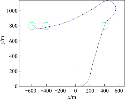
Fig. 7 Vessel course in x-y graph while it has speed of 7 m/s

Figure 8(a) shows the actual heading angle and the Kalman filter estimation of yaw angle of the controlled vessel which is between [-180° +180°]. Figure 8(b) depicts the rudder angle. As seen in this figure, the estimated yaw angle is very similar to the actual yaw angle of the vessel. In this figure, the rudder angle has low motion at the wave frequency thanks to the effect of the wave filtering. In other words, because only the low-frequency estimates of the heading angle and rate produced by the Kalman filter are passed to the controller, the motion of the rudder is not be influenced by wave motion, and thus wave filtering is achieved.

Figure 9 shows the value of the vessel roll angle in the wave field. As seen in the figure, roll angle of the vessel is relatively high in the presence of wave loads. Roll motion controlling of marine vessels has been a representative control problem for marine applications and has attracted considerable attention from the control community [21].

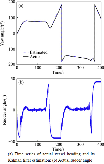
Fig. 8 Performance of heading autopilot in the presence of wave loads:

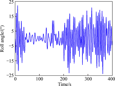
Fig. 9 Roll angle of vessel in wave field

To evaluate the effect of wave-inducted roll motion, a straight line scenario is defined. The initial condition of the vessel and the other wave and sensor parameters are the same with the previous example. Figure 10(a) shows the roll of the vessel in the straight course. As seen in this figure the amount of the roll of the vessel is relatively high. Figure 10(b) depicts the yaw angle which is near zero proving the straight course of the vessel. Figure 10(c) shows the rudder angle. As expected, the rudder angle is near zero to keep the vessel in the straight line. In this condition the roll angle cannot be affected by the rudder motion. It means that the roll angle is majorlyaffected by the wave-inducted moments. The vessel can also be equipped with auxiliary fin devices to control roll motion of the vessel, especially in wave fields that makes a multi-input control problem.

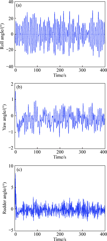
Fig. 10 Roll (a), yaw (b) and rudder (c) angles of vessel in straight line course

To evaluate the robustness of the controller and observer at different conditions, the first scenario is repeated with a different vessel speeds. Assume that the vessel has the constant speed of 15 m/s during the course. The other initial conditions and LOS waypoints are the same with the first scenario. Figure 11 shows the vessel course in x-y graph. As seen in this figure, the vessel moves toward 3 waypoints. Figure 12(a) shows the roll of the vessel. Figure 12(b) depicts the yaw angle of the vessel. Figure 12(c) shows the rudder angle. In this example the vessel is located within the waypoints in less time than the first scenario due to higher speed of the vessel. While the controller is designed for the nominal speed of 7 m/s, the design is robust even in the speed of 15 m/s. This is especially important for speed-varying manoeuvres.

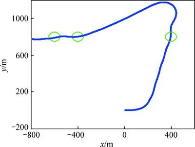
Fig. 11 Course of vessel in x-y graph while it has speed of 15 m/s

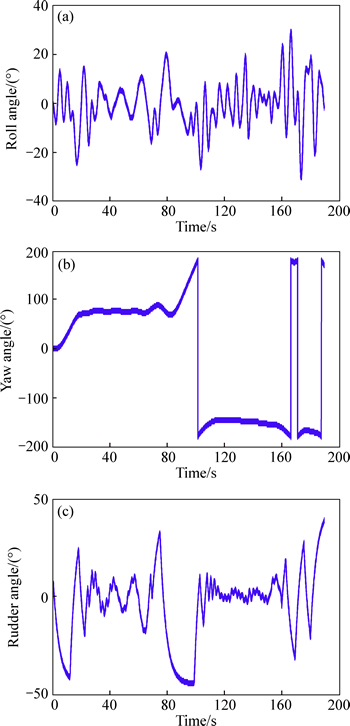
Fig. 12 Roll (a), yaw (b) and rudder angles (c) of vessel in last scenario

5 Conclusion and closing remarks

In this work a transfer function model for roll and yaw dynamics of a container ship, based on the Nomoto model, using CIFER software has been derived. Based on the identified Nomoto constants, a PID heading controller has been designed and a reference model has been added to the controller to achieve accurate course-changing manoeuvres. A Kalman filter observer based on the identified Nomoto model has also been designed for wave filtering as well as estimating states of the vessel. To illustrate the performance of the designed observer case studies for line of sight waypoint guidance of the vessel were considered. Results show that the proposed identification method results in an accurate state estimation and control the vessel toward waypoints while filtering the external waves. It is also shown that the controller and observer are robust in different vessel speeds. These case studies show the capability of CIFER software to identify marine vessel’s dynamics and open a new window to verify the effectiveness of the presented technique in real application.

References

[1] KLLSTRM C G, K J. Experiences of system identification applied to ship steering [J]. Automatica, 1981, 17: 187-198.

[2] HOLZHUTER T. Robust identification scheme in an adaptive track controller for ships [C]// 3rd IFAC Symp Adaptive Systems in Control and Signal Processing. Glasgow, 1989: 118-123.

[3] HADDARA M, WANG Y. Parametric identification of manoevring models for ships [J]. Int Shipbuild Progr, 1999, 46: 5-27.

[4] ZHANG X G, ZOU Z J. Identification of Abkowitz model for ship manoeuvring motion using ε-support vector regression [J]. Journal of Hydrodynamics, 2011, 23: 353-360.

[5] SELVAM, R P, BHATTACHARYYA, S K, HADDARA M A. frequency domain system identification method for linear ship maneuvering [J]. Int Shipbuild Progr, 2004, 52: 5-27.

[6] TISCHLER M B, REMPLE R K. Aircraft and rotorcraft system identification: Engineering methods with flight-test examples [S]. American Institute of Aeronautics and Astronautics, 2006.

[7] NOMOTO K, TAGUCHI T, HONDA K, HIRANO S. On the streeing qualities of ships [J]. Int Shipbuild Progr, 1957, 4.

[8] ASADI M, NARM H G. Adaptive stochastic sliding mode ship autopilot for way-point tracking [C]// 21st Iranian Conference on Electrical Engineering (ICEE). Mashhad, 2013: 1-6.

[9] CAHARIJA W. Integral line-of-sight guidance and control of underactuated marine vehicles [R]. 2014.

[10] LIU L, WANG D, PENG Z. Path following of underactuated MSVs with model uncertainty and ocean disturbances along straight lines [C]// Control and Decision Conference (CCDC). Osaka, 2015: 2590-2595.

[11] PEYMANI E, FOSSEN T I. Path following of underwater robots using Lagrange multipliers [J]. Robotics and Autonomous Systems, 2015, 67: 44-52.

[12] ZHENG H, NEGENBORN R R, LODEWIJKS G. Trajectory tracking of autonomous vessels using model predictive control [C]// 19th IFAC World Congress. Cape Tocvn, South Africa, 2014.

[13] FOSSEN T I. Guidance and control of ocean vehicles [M]. West Sussex, England: Wiley, 1994.

[14] YOUNG P, PATTON R J. Comparison of test signals for aircraft frequency domain identification [J]. J Guidance, Control, and Dynamics,1990, 13: 430-438.

[15] OPPENHEIM A V, SCHAFER R W. Discrete-time signal processing [M]. 3rd ed. Upper Saddle River, NJ: Prentice-Hall, 2010.

[16] VANREUSEL S. Identification and multivariable feedback control of the vibration dynamics of an automobile suspension [D]. Montreal: Dept. Elec Eng, Mc Gill Univ, 2005.

[17] MOREIRA L C, FOSSEN T I, SOARES C G. Path following control system for a tanker ship model [J]. Ocean Engineering, 2007, 34: 2074-2085.

[18] FOSSEN T I. Handbook of marine craft hydrodynamics and motion control [M]. UK: John Wiley & Sons, 2011.

[19] LI Z. Path following with roll constraints for marine surface vessels in wave fields [D]. Michigan: Naval Architecture and Marine Engineering, University of Michigan, 2009.

[20] FALTINSEN O M. Sea loads on ships and offshore structures [M]. Cambridge, UK: Cambridge University Press, 1990.

[21] PEREZ T, BLANKE M. Ship roll motion control [C]// The IFAC CAMS. Rostock-Warnemunde, Germany, 2010.

(Edited by YANG Hua)

Received date: 2015-06-25; Accepted date: 2015-11-13

Corresponding author: M. T. Ghorbani, PhD Candidate; Tel: +351-21-841-8088; E-mail: mohammadtaghi@isr.ist.utl.pt