J. Cent. South Univ. (2012) 19: 347-356

DOI: 10.1007/s11771-012-1011-8

Effects of groove on behavior of flow between hydro-viscous drive plates

HUANG Jia-hai(黄家海)¹, FAN Yu-run(范毓润)¹, QIU Min-xiu(邱敏秀)¹, FANG Wen-min(方文敏)²

1. State Key Laboratory of Fluid Power Transmission and Control, Zhejiang University, Hangzhou 310027, China;

2. The Third Department PLA Artillery Academy, Hefei 230031, China

? Central South University Press and Springer-Verlag Berlin Heidelberg 2012

Abstract: The flow between a grooved and a flat plate was presented to investigate the effects of groove on the behavior of hydro-viscous drive. The flow was solved by using computational fluid dynamics (CFD) code, Fluent. Parameters related to the flow, such as velocity, pressure, temperature, axial force and viscous torque, are obtained. The results show that pressure at the upstream notch is negative, pressure at the downstream notch is positive and pressure along the film thickness is almost the same. Dynamic pressure peak decreases as groove depth or groove number increases, but increases as output rotary speed increases. Consequently, the groove depth is suggested to be around 0.4 mm. Both the groove itself and groove parameters (i.e. groove depth, groove number) have little effect on the flow temperature. Circumferential pressure gradient induced by the groove weakens the viscous torque on the grooved plate (driven plate) greatly. It has little change as the groove depth increases. However, it decreases dramatically as the groove number increases. The experiment results show that the trend of experimental temperature and pressure are the same with numerical results. And the output rotary speed also has relationship with input flow rate and flow temperature.

Key words: hydro-viscous drive; variable viscosity; groove effect; numerical calculation

1 Introduction

Hydro-viscous drive transfers power with viscous shearing force. The output angular velocity can be regulated by changing the clearance between plates. During the state of output rotary speed regulation, the gap between plates is filled with transmission oil. This oil provides lubrication and carries lots of heat away. It is not necessary to groove on the plate face in theory. But in practice, the hydro-viscous plate surfaces are sometimes deliberately grooved to avoid the thermal deformation of plate induced by local contact.

PAYVAR et al [1-2] analyzed that the heat transfers to laminar flow in radial grooves of wet clutch friction faces. BERGER et al [3] investigated the effects of applied load, friction material permeability and groove geometry on the engagement characteristics of wet clutch. The results showed that the wider grooves increase the engagement time, and groove depth has little effect on engagement characteristics. The squeezing film flow between plates in wet clutch was solved numerically by RAZZAQUE and KATO [4]. The results indicated that grooves inclined with the flow direction result in less viscous torque. YUAN et al [5] developed a 3D, steady-state, two-phase flow model for the flow in the disengaged wet clutch pack to investigate the effects of rotary speed of friction plates, gap and flow rate on disengaged drag torque and power loss. YUAN et al [6] also investigated the hydrodynamic behavior of flow in a disengaged wet clutch under the consideration of surface tension effect.

WEI and ZHAO [7] gave a detailed introduction about hydro-viscous drive. CHEN [8] investigated the thermal stress and thermal deformation of plates in hydro-viscous drive. HONG et al [9] investigated the engagement of wet clutch with rectangular grooves. HUANG et al [10] conducted some computational studies on the flow between plates in hydro-viscous drive and analyzed the distribution of temperature and pressure, but this work did not point out the effect of groove on the viscous torque.

MENG and HOU [11] reported that the grooves in hydro-viscous soft start are the formation basis of dynamic pressure but they may reduce the capacity of torque transfer to a certain extent during startup  process. MASATOSHI et al [12] concluded that the temperature at the friction plate surface can be controlled effectively by radial grooves in combination with circumferential ones during the engagement of wet clutch.

The flow between plates in wet clutch during disengaged mode was solved numerically by APHALE  et al [13]. But their work did not consider the effect of temperature on viscosity and the effect of circumferential pressure gradient on viscous torque. APHALE et al [14] investigated new groove geometry to study its efficiency in promoting aeration between plates in wet clutch during the disengaged mode.

Summarizing the previous works, the squeezing flow between plates and the effect of grooves on engagement characteristics are well understood. However, few works are focused on the effects of the groove depth and groove number on the flow between plates when the gap is constant.

The objective of this work is to investigate the effect of groove on the behavior of hydro-viscous drive (including viscous torque, axial force, temperature and pressure) in a steady rotary speed regulation mode, namely, the clearance is constant. Then, the effect of groove depth and groove number (ratio of the grooved area to the total plate surface area is constant) on the hydro-viscous drive is presented. The experimental study on the output rotary speed under different input flow rates and temperature conditions are carried out.

2 Physical model

The physical model of flow between plates is depicted schematically in Fig. 1. Only a part of the flow containing one groove is taken because of its periodicity. The clearance between plates is h₀. The flat driving plate (lower plate) rotates at a constant angular speed ω₁ and the grooved upper plate (driven plate) rotates at an angular speed ω₂. The driven plate has n radial grooves on its working surface. The angular span of the groove is α, and the groove depth is h_gro. For convenience, the computational domain is treated in (r, θ, z) cylindrical coordinate system. θ=0 and θ=φ are the periodic boundaries in circumferential direction. The mark “inlet” denotes the input boundary and “outlet” denotes the output boundary.

2.1 Governing equations

The following assumptions are made in the analysis of the flow in hydro-viscous drive:

1) The flow is steady, laminar and incompressible Newtonian fluid. All physical properties remain constant except variable viscosity with temperature.

2) No slip occurs at fluid/solid interfaces.

3) Body force and inertial forces except centrifugal force are negligible.

4) Surface roughness of plates is negligible.

5) Cavitation does not occur.

6) The gradients of velocity in the axial are much more important than radial velocity gradients, namely:

where V_θ, V_r, V_z are tangential, radial and axial velocity components respectively; r, θ, z are axes of cylindrical coordinates, respectively.

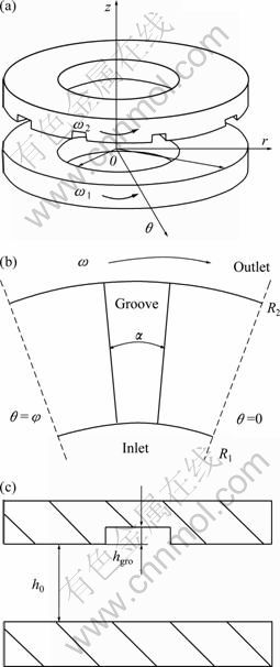
Fig. 1 Physical model of plates

Continuity equation:

Momentum equations:

where ρ is the oil density, p is the pressure, and μ is the dynamic viscosity of fluid.

The wall boundary conditions for Eqs. (1)-(4) are

where ω₁ and ω₂ are angular velocities of the driving plate and driven plate, respectively.

Periodic boundary condition is

The variable viscosity with temperature makes the momentum equation couple with energy equation. As a result, the energy equation is required in addition to  Eqs. (1)-(4).

Energy equation is

where T is the temperature.

Boundary conditions for Eq. (7) are

Integrating Eq. twice with respect to z, substitution of the boundary condition Eq. is

Shear stress acting on the driving plate and driven plate can be calculated respectively:

where t_zq is the shear stress acting on the plate.

Viscous torque acting on the plate as expressed in Eqs. and is determined by integrating Eqs. and over the surface area, respectively:

where M₁ is the viscous torque acting on the driving plate, M₂ is the viscous torque acting on the driven plate, β is the ratio of the grooved area to total area, and n is the number of grooves.

The difference between the driving plate and the driven plate is

It can be found from Eqs. - that the

circumferential pressure gradient  induced by the

groove increases the shear stress and viscous torque on the driving plate, but decreases them on the driven plate

when . In particular, this effect on the driven

plate is more significant. Equations and also express that the viscous torque on the driving/driven plate has relations with the ratio of the grooved area to the total surface area.

The axial force is

where F is the axial force acting on the driving or driven plate.

2.2 Viscosity-temperature equation

Viscosities of 6^# hydrodynamic transmission oil at different temperatures were carried out on a rheometer (Gemini 200 rheometer, Bohlin Co., UK) with parallel plate geometry (25 mm in diameter). All measurements were conducted at a standard atmospheric pressure. Temperature sweeps with 5 °C increment from 25 °C to 100 °C.

The fitting curve of viscosity versus temperature based on ERING [15] model and experimental viscosities are shown in Fig. 2. The viscosity versus temperature equation is

Fig. 2 Curve fit of viscosity-temperature equation

3 Numerical computation

The energy equation is coupled with momentum equation each other due to variable viscosity with temperature. As a result, momentum and energy equations could not be solved analytically, even though they have been simplified in Section 2.1. Consequently, the flow is solved numerically by using computational fluid dynamics (CFD) code Fluent based on finite volume method [16] (FVM) in this case. The grid files of geometries listed in Table 1 were generated by using structured grid with hexahedral mesh elements in Gambit. In order to make the computation domain approach the real flow, fluid region marked with letter A as shown in Fig. 3 is also included in the computation domain. boundary conditions were specified according to Eq. in Section 2.1. Similarly, the thermal boundary conditions were specified on the basis of Eqs. , and . Pressure gradient at the periodic boundary θ=0 and θ=φ was assigned to be zero, and the temperature at the periodic boundary was specified according to     Eq. . The boundary marked with “inlet” as shown in Fig. 3 was specified as velocity inlet boundary condition. The boundary marked with “outlet” was specified as pressure outlet boundary condition, and the pressure value was assigned to be zero.  Pressure–velocity coupling was resolved by means of SIMPLEC algorithm. The second order upwind was used for the momentum and energy equations.

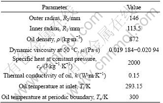
Table 1 Geometry parameters

The gird file was then imported into Fluent. The solver and parameters related to numerical computation as listed in Table 2 were specified in Fluent. The wall

Fig. 3 Grid of n =15, h_gro= 0.2 mm, h = 0.1 mm, α = 4.5° and  β = 18.75%

Table 2 Parameters for computation

4 Results and discussion

Figure 4 shows the pressure contour in the domain (113.5 mm ≤ r ≤ 146 mm, 0° ≤ θ ≤ 24°). The pressure along the film thickness (z direction) is almost uniform,

namely, . The flow section in circumferential

direction expands and narrows suddenly due to the groove. In order to satisfy the continuity of flow, pressure at the upstream notch decreases to negative pressure and pressure at the downstream notch creates a higher positive pressure owing to the incompressibility of oil.

To check the accuracy of the numerical results, energy balance among results is conducted as follows. The power difference between the driving plate and the driven plate is compared with total heat transfer rate in computation domain. If the error is very small, it means that numerical results are correct. For example, in Fig. 4, the viscous torques on the driving plate and driven   plate are M₁=1.704 428 N·m and M₂=0.931 5 N·m, respectively. So, the power difference is M₁ω₁–M₂ω₂= 188.37 W. The numerical total heat transfer rate in Fluent is 187.563 07 W. It is obvious that the numerical results are correct.

Fig. 4 Pressure contour for ω₁ = 149 5 r/min, ω₂ = 800 r/min,  n =15, h = 0.1 mm, h_gro= 0.2 mm, α = 4.5° and Q = 1.5 L/min

Increasing the output rotary speed ω₂ leads to the increase in the hydrodynamic pressure peak induced by grooves as shown in Fig. 5(a), and the negative pressure peak is smaller than the positive pressure peak. It is clear that cavitation is more likely to occur as hydrodynamic negative pressure peak increases. Figure 5(b) shows that fluid temperature T decreases as ω₂ increases. At the same radius, T at the upstream region (θ ≥14.5°) is lower than that at the downstream region (θ≤10°). Furthermore, T reaches its maximum at θ=10° and arrives at its minimum at θ=14.5°. Figure 6(a) depicts that viscous torque acting on the driving plate M₁ is higher than that on driven plate M₂. Besides that, both M₁ and M₂ decrease as ω₂ increases, but ΔM (ΔM=M₁-M₂) increases with increasing ω₂. This is because the circumferential pressure gradient increases as ω₂ increases as shown in Fig. 5(a), which results in the increment of ΔM. The axial force that acting on the plate with grooves is lower than F acting on the flat plate, as shown in Fig. 6(b).

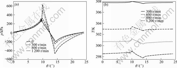
Fig. 5 Numerical results for ω₁=1 495 r/min, Q=1.5 L/min, h=0.1 mm, n =15, h_gro=0.2 mm, α=4.5°, r=140 mm and z=0.05 mm:    (a) Pressure distribution; (b) Temperature distribution

Fig. 6 Numerical results for ω₁=1 495 r/min, Q=1.5 L/min, h=0.1 mm, n=15, h_gro=0.2 mm, α=4.5°, r=140 mm and z= 0.05 mm:    (a) M₁, M₂, DM; (b) F

4.1 Effect of groove depth

The velocity contours show a decrease in fluid velocity at the non-grooved region (θ≤10° and θ≥14.5°) with increasing the groove depth h_gro, as depicted in  Fig. 7. And the fluid velocity in the groove (10°≤θ≤ 14.5°) increases as h_gro increases. Figure 8(a) shows that the hydrodynamic (negative) pressure peak decreases as h_gro increases. The increment of h_gro means that the right hand side term in Eq. (3) decreases. So, the hydrodynamic pressure peak decreases accordingly. In Fig. 8(b), when h_gro≤0.3mm, T increases as h_gro increases in non-grooved region (θ≤10° and θ≥14.5°) and changes reversely in the groove (10°≤θ≤14.5°). However, when h_gro≥0.4mm, T decreases as h_gro increases. But the  extent of decrease in T is very limited. Figure 9(a) shows that F decreases as h_gro increases when input flow rate  Q is constant. F increases as ω₂ increases when  h_gro=0.1 mm. However, it almost does not vary with ω₂ when h_gro≥0.2 mm. In other words, F can be defined as a constant when h_gro≥0.2 mm. Figure 9(b) expresses that the increase in h_gro has little effect on viscous torque.

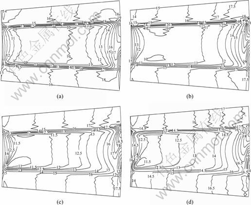
Fig. 7 Velocity distributions for ω₁=1 495 r/min, n=15, h=0.1 mm, α=4.5°, z=0.05 mm, ω₂=800 r/min and Q=1.5 L/min: (a) h_gro=  0.1 mm; (b) h_gro=0.2 mm; (c) h_gro=0.3 mm; (d) h_gro=0.4 mm

Fig. 8 Numerical results for ω₁=1 495 r/min, n=15, h=0.1 mm, α=4.5°, ω₂= 800 r/min, Q=1.5 L/min, r=140 mm and z=0.05 mm:   (a) Pressure distribution; (b) Temperature distribution

It can be inferred from Figs. 8 and 9 that the optimum groove depth is suggested to be around 0.4 mm. This is mainly because the negative pressure peak caused by the groove can be reduced effectively with increasing the h_gro. So, increasing the groove depth is an effective way to prevent cavitation happening. However, once h_gro≥0.4 mm, the hydrodynamic (negative) pressure peak decreasing rate will become very slow. In addition, the increment of h_gro has little effect on the viscous torque and flow temperature.

4.2 Effect of number of grooves

When β = 18.75%, the increase in groove numbers n results in the decrement of the pressure peak and fluid temperature, as shown in Fig. 10. This is because the angular span of the groove α decreases as n increases when β remains constant. It can be inferred from Eq. (3) that pressure will be reduced by decreasing α when other parameters remain constant. In contrary to that, the axial force acting on the plate as depicted in Fig. 11(a) increases as n increases. It is noteworthy that M₂ decreases as n increases, as shown in Fig. 11(b). M₂ is very little when n=90. However, an increase in n has little effect on M₁. The reason for above is that the circumferential pressure gradient increases as n increases as shown in Fig. 10(a). According to Eqs. (13)-(16), the increment of the circumferential pressure gradient will result in the decrement of M₂.

5 Experimental apparatus and results

5.1 Apparatus and measurements

Figure 12 shows a sketch of the experimental rig. The experimental hydro-viscous drive consisted of a driving plate (flat plate) and a radially-grooved driven plate. The driven plate had 15 equally distributed grooves (α=12°, h_gro=0.4 mm) on its working surface. Oil was forced into the gap between plates through the oil entrance and exited at the outside diameter. The input rotary speed and torque were measured with transducer, and output rotary speed and torque were measured with transducer. The sampling interval of transducers was set as 3 s. The clearance between plates was adjusted and locked by nuts. The thickness of the fluid film was measured with two eddy current displacement sensors (linear measurement range: 0.31-2.31 mm). The inlet oil temperature was measured by means of platinum resistance temperature sensor Pt100 (probe diameter:   3 mm, measurement range: 0-100 °C). The input flow rate was measured with turbine flow sensor.

Fig. 9 Numerical results for ω₁=1 495 r/min, n=15, h=0.1 mm, α=4.5° and Q=3 L/min: (a) F; (b) M₁, M₂

Fig. 10 Numerical results for different groove numbers when ω₁=1 495 r/min, ω₂=800 r/min, h=0.1 mm, h_gro=0.2 mm, Q=3 L/min, r=140 mm and z=0.05 mm: (a) Pressure distribution; (b) Temperature distribution

Fig. 11 Numerical results for different groove numbers when ω₁=1 495 r/min, ω₂=800 r/min, n=15, h=0.1 mm, h_gro=0.2 mm and Q = 3 L/min: (a) F; (b) M₁, M₂

Fig. 12 Sketch of hydro-viscous drive experimental rig:       1—Motor; 2, 6—Torque and rotational speed measuring device; 3—Adjustment and lock nuts; 4—Driving plate; 5—Driven plate; 7—Magnetic power brake; 8—Eddy current displacement sensor; 9—Data acquisition card; 10—Personal computer

In order to facilitate installation of temperature and pressure transducers, the driven plate was fixed still in the test rig during the measurement of oil temperature and pressure between plates. The probes were installed in the driven plate, as shown in Fig. 13. Temperature at the points marked with T1, T2 were measured with platinum resistance temperature sensor Pt100. The Pt100 was mounted in Teflon insert which was screwed into the carbon steel driven plate. The pressure at the points marked with P1, P2, P3 were measured by means of dynamic pressure transducers.

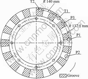
Fig. 13 Installation diagram of temperature and pressure transducers in driven plate

5.2 Experimental results

Figure 14 shows the theoretical and experimental temperature at points T1, T2 for different input rotary speed ω₁. It can be seen that temperature at T1, T2 increases as ω₁ increases. It is also shown that the temperature at the point T2 in the groove is lower than that at T1 in the non-grooved area. When ω₂=0, Q=    2 L/min and h=0.082 mm, the numerical pressure (ω₁=500 r/min), experiment static pressure (ω₁=0) and experiment hydrodynamic pressure (ω₁=500 r/min) are shown in Fig. 15. It can be seen that experimental pressure at point P2, P3 under static and dynamic conditions are almost the same as the numerical results, and experimental pressure at P1 under dynamic condition increases greatly. The trend of experimental pressure under dynamic condition is the same as the numerical results, but the numerical result at P1 is higher than the experimental one, as shown in Fig. 15. One possible reason is that the installation of dynamic pressure transducer has an effect on the development of experiment dynamic pressure. Another one is that the pressure measured by dynamic pressure transducers represents the average pressure of cross section rather than a point.

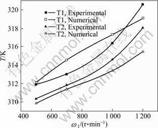
Fig. 14 Experimental and numerical temperature at T1, T2 when ω₂= 0, Q=2 L/min and h=0.066-0.102 mm

Fig. 15 Experiment and numerical pressures at P1, P2 and P3 for ω₁=500 r/min, ω₂=0, Q=2 L/min and h=0.066-0.102 mm

Experimental output angular velocity ω₂ is shown in Fig. 16. It can be concluded from Fig. 16 that the input flow temperature T_i has an important effect on ω₂ when ω₁, h and M₂ remain constant. The ω₂ decreases linearly as T_i increases and increases as input flow rate Q increases. Figure 17 shows that the fitting curve of ω₂ under h=0.078-0.114 mm condition is approximately parallel to that under h = 0.165-0.252 mm. And ω₂ under h=0.078-0.114 mm is higher than that under h= 0.165-0.252 mm. Figure 18 depicts the relation between M₂ and ω₂ when ω₁ remains constant. It can be found that M₂ has an approximately linear relation with ω₂ when ω₂ ≥ 400 r/min.

Fig. 16 Experimental output rotary speed under different inlet flow temperatures and different input flow rates when ω₁=    1 495 r/min, h=0.078-0.114 mm and M₂≈0.8 N·m

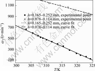
Fig. 17 Experimental output rotary speed under ω₁=1 495 r/min, Q=5.5 L/min and M₂≈0.8 N·m

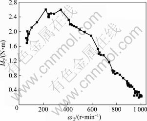
Fig. 18 Experimental output rotary and torque when ω₁=  1 495 r/min, Q=6 L/min, h=0.22-0.269 mm and T_i=302.15- 305.15 K

6 Conclusions

1) The viscous torque and axial force acting on the grooved driven plate are decreased by the grooves compared with that acting on the flat driven plate. But the grooves have little effect on the fluid temperature between plates in hydro-viscous drive.

2) The increment of groove depth has little effect on the fluid temperature and the viscous torque acting on the driving and driven plate. However, increasing the groove depth results in the decrease in axial force and dynamic negative pressure peak that can induce the generation of cavitation, but once the groove depth is more than    0.4 mm, pressure peak and axial force decreasing rate become slow; consequently, the groove depth is suggested to be around 0.4 mm.

3) Dynamic pressure peak, flow temperature and viscous torque acting on the driven plate decrease as groove number increases when the ratio of the grooved area to total area of plate is constant. However, the axial force increases as groove number increases.

4) Experimental results show that the trends of experimental temperature and pressure are the same as the numerical results. This means that the numerical method presented here is a feasible way to predict the flow between plates in hydro-viscous drive under the condition of constant clearance.

References

[1] PAYVAR P. Laminar heat transfer in the oil groove of a wet clutch [J]. International Journal of Heat and Mass Transfer, 1991, 34(7): 1791-1797.

[2] PAYVAR P, LEE Y N, MINKOWYCZ W J. Simulation of heat transfer to flow in radial grooves of friction pairs [J]. International Journal of Heat and Mass Transfer, 1994, 37(2): 313-319.

[3] BERGER E J, SADEGHI F, KROUSGRILL C M. Finite element modeling of engagement of rough and grooved wet clutches [J]. ASME Journal of Tribology, 1996, 118: 137-145.

[4] RAZZAQUE M M, KATO T. Effects of a groove on the behavior of a squeeze film between a grooved and a plain rotating annular disk [J]. ASME Journal of Tribology, 1999, 121: 808-815.

[5] YUAN Y Q, ATTIBELE P, DONG Y. CFD simulations of the flows within disengaged wet clutches of an automatic transmission [R]. 2003-01-0320.

[6] YUAN Y Q, LIU E A, HILL J, ZOU Q. An improved hydrodynamic model for open wet transmission clutches [J]. ASME Journal of Fluids Engineering, 2007, 129: 333-337.

[7] WEI Cheng-guan, ZHAO Jia-xiang. Hydro-viscous transmission technology [M]. Beijing: National Defence Industry Press, 1996: 51-80. (in Chinese)

[8] CHEN Ning. Theoretical and application researches on hydroviscous drive [D]. Zhejiang University, 2003. (in Chinese)

[9] HONG Yue, LIU Bao-yun, JIN Shi-liang, YIN Zhe-hao. The engagement of the friction coupling of wet clutch with groove [J]. Lubrication Engineering, 2007, 32(12): 69-73. (in Chinese)

[10] HUANG Jia-hai, QIU Min-xiu, LIAO Ling-ling, FU Lin-jian. Numerical simulation of flow field between frictional pairs in hydroviscous drive surface [J]. Chinese Journal of Mechanical Engineering, 2008, 21(3): 72-75.

[11] MENG Qing-rui, HOU You-fu. Mechanism of hydro-viscous soft start of belt conveyor [J]. Journal of China University of Mining & Technology, 2008, 18(3): 459-465.

[12] MASATOSHI M, MASATAKA O, YASUNORI O, HIROKI H, SHINOBU S, KAZUYUKI O. Numerical simulation of temperature and torque curve of multidisk wet clutch with radial and circumferential groove [J]. Tribology Online, 2009, 4(1): 17-21.

[13] APHALE C R, CHO J, SCHULTZ W W, CECCIO S L, YOSHIOKA T, HIRAKI H. Modeling and parametric study of torque in open clutch plates [J]. ASME Journal of Tribology, 2006, 128: 422-430.

[14] APHALE C R, SCHULTZ W W, CECCIO S L. The influence of grooves on the fully wetted and aerated flow between open clutch plates [J]. ASME Journal of Tribology, 2010, 132: 1-7.

[15] BYRON B R, STEWART W E, LIGHTFOOT E N. Transport phenomena [M]. New York: John Wiley & Sons, Inc, 1960.

[16] PATANKAR S V. Numerical heat transfer and fluid flow [M]. Washington: Hemisphere, 1980: 41-137.

(Edited by YANG Bing)

Foundation item: Project(50475106) supported by the National Natural Science Foundation of China

Received date: 2010-09-19; Accepted date: 2011-01-10

Corresponding author: HUANG Jia-hai, PhD candidate; Tel: +86-571-87951314-6206; E-mail: huangjh79@gmail.com