J. Cent. South Univ. (2012) 19: 2520-2527

DOI: 10.1007/s11771-012-1305-x

Element yield rate prediction in ladle furnace based on improved GA-ANFIS

XU Zhe(徐喆)^{1, 2}, MAO Zhi-zhong(毛志忠)^{1, 2}

1. School of Information Science and Engineering, Northeastern University, Shenyang 110819, China;

2. State Key Laboratory of Integrated Automation for Process Industries (Northeastern University), Shenyang 110819, China

? Central South University Press and Springer-Verlag Berlin Heidelberg 2012

Abstract: The traditional prediction methods of element yield rate can be divided into experience method and data-driven method. But in practice, the experience formulae are found to work only under some specific conditions, and the sample data that are used to establish data-driven models are always insufficient. Aiming at this problem, a combined method of genetic algorithm (GA) and adaptive neuro-fuzzy inference system (ANFIS) is proposed and applied to element yield rate prediction in ladle furnace (LF). In order to get rid of the over reliance upon data in data-driven method and act as a supplement of inadequate samples, smelting experience is integrated into prediction model as fuzzy empirical rules by using the improved ANFIS method. For facilitating the combination of fuzzy rules, feature construction method based on GA is used to reduce input dimension, and the selection operation in GA is improved to speed up the convergence rate and to avoid trapping into local optima. The experimental and practical testing results show that the proposed method is more accurate than other prediction methods.

Key words: genetic algorithm; adaptive neuro-fuzzy inference system; ladle furnace; element yield rate; prediction

1 Introduction

In the competitive market scenario, steel producers are striving for high-speed continuous casting with stringent and consistent quality as well as reduced production cost. The ladle furnace (LF) is a key unit for achieving the above objectives during refining process. In alloying process of LF, alloys are added in appropriate proportion to liquid steel, which will cause the change of the element concentrations in steel. The yield rates of alloy elements are key parameters to the alloy addition in LF alloying process. It can be defined as the ratio of changing quantity of one element in liquid steel to the total quantity of the same element added into the molten steel. Because of complex physical and chemical reactions in LF process, the accurate mechanism prediction model cannot be established. Therefore, a soft-sensor model can be used for the prediction. The studies of soft-sensor modeling for element yield rate predicting in LF can be divided into two methods: experience method and data-driven method. The experience method is based on the rule of thumb developed through operating experience. Reference heat method was presented by YU et al [1], which gets the current yield rates by using average values of the yield rates of reference heats. Similarly, ladle furnace on-line reckoner (LFOR) was proposed by NATH et al [2], which uses empirical formulae to calculate the yield rates. But, because of the low adaptation ability, experience method is restricted to certain production environments, and small variations can lead to the inaccurate prediction values.

With development and wide application of artificial intelligence in industry, GAO et al [3] used neural network to overcome above limitations. But the prediction accuracy of this data-driven method is afflicted with insufficient sample dataset. To cover this shortage, an improved adaptive neuro-fuzzy inference system (ANFIS) is proposed, in this work, which incorporates human knowledge (in the form of fuzzy if-then rules) into ANFIS as compensation for insufficient training data.

Because there are a lot of measurable data, in order to facilitate the experience incorporation and acquisition of intelligible fuzzy rules, dimension reduction method is needed. But, the commonly-used dimension reduction methods, such as feature selection [4] and feature extraction [5-6], are not suitable for this problem. As to feature selection, features of high importance can be selected, but other features that are still useful will be ignored. The way of feature extraction could not keep the original physical meanings of inputs, which is important for fuzzy system. To solve this problem, feature construction method based on improved genetic algorithm (GA) [7-9] is proposed, which can retain more information and keep certain physical interpretations of the constructed features.

Specifically, the contributions of this work include:

1) The mechanism analysis is carried out to determine the features needed to be constructed and the relationships between these features and the measurable variables.

2) A feature construction method based on GA is proposed. According to the mechanism analysis, the constructed features obtained by this method are easily interpretable, and can provide the quantitative evaluation of interest. Moreover, the selection operation in GA has been improved so as to accelerate the convergence rate and avoid trapping into local optima.

3) The ANFIS method is improved so as to model with both empirical knowledge and data samples.

2 Mechanism analysis

Through mechanism analysis of refining process, main factors affecting element yield rates in LF can be determined as follows: concentration of dissolved oxygen, concentrations of iron oxide and manganese oxide in slag, slag basicity, effect of argon stirring and temperature of molten steel [10]. But the values of these factors cannot be obtained when making predictions. To solve this problem, new features according to the affecting factors can be constructed by using the measurable variables.

The measurable variables and sampling times in LF refining process are shown in Fig. 1.

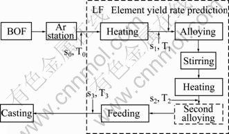
Fig. 1 Measurable variables and sampling times in LF refining process

In Fig. 1, s₀ and T₀ are the composition and temperature samples before ladle enters LF station. s₁ and T₁ are the first composition and temperature samples in LF station, and predictions can be carried out after s₁ is obtained. s₂ and T₂ are the second composition and temperature samples in LF station. If s₂ does not meet the production requirements, a second alloying process is needed. s₃ and T₃ are the last composition and temperature samples in LF station.

The relationships between the main factors and the measurable variables are as follows:

1) Concentration of dissolved oxygen (F₁)

Due to the expensive detecting cost, concentration of dissolved oxygen is rarely detected in practice. However, the element contents (mass fraction, %) of Si (w₀(Si)), Mn (w₀(Mn)) and Al (w₀(Al)) in s₀ can be used to measure the concentration of dissolved oxygen, indirectly.

2) Concentrations of iron oxide and manganese oxide in slag (F₂)

It mainly refers to the concentrations of FeO and MnO in slag. For Si-killed steel, the related variables are the rates of concentration change of C (Δw(C)/t_s= (w₁(C)-w₀(C))/t_s), Mn (Δw(Mn)/t_s=(w₁(Mn)–w₀(Mn))/t_s), and Si (Δw(Si)/t_s=(w₁(Si)-w₀(Si))/t_s), masses of added carbon powder (m_C) and ferrosilicon powder (m_S). t_s is the time span between the time when refining process starts and s₁ is obtained.

3) Slag basicity (F₃)

It is the ratio of the content of basic oxide to the content of acidic oxide in slag. The related variables are as follows: the rate of content change of S (Δw(S)/t_s=(w₁(S)-w₀(S))/t_s), initial content of S (w₀(S)), mass of added fluorite (m_F) and lime (m_L).

4) Effect of argon gas bottom stirring (F₄)

It is related to the argon volume flow-rate of each stage in refining process. The argon volume flow-rates are determined by argon blowing system, and the blowing system is mainly affected by w(S)₁, mass of liquid steel (m_t) and the time of refining cycle (t_c). In addition, the waving level of the liquid steel surface can be used to measure the intensity of argon stirring indirectly. If the stirring is vigorous, the liquid steel surface will be churned violently, and can be exposed to the atmosphere, which can result in the secondary oxidation of alloy elements. The arc-impedances are changed with the fluctuation of liquid steel surface; therefore, the arc-current fluctuation is in direct proportion to the fluctuation of liquid steel surface. The average value of arc-current fluctuation (P_D) of three phases, as shown in Eq. , can be used to measure the fluctuation level of liquid steel surface. The standard deviation of the arc-current of phase A (D_A) is defined in Eq. (2):

where  is the arc-current of phase A at time i; n is the number of sampling arc-current values of phase A;  is the average arc-current of phase A;  and D_C can be calculated in the same way.

5) Temperature of molten steel (F₅)

For the oxidation reaction is exothermic, the oxidation of alloy element decreases with an increase in temperature. It can be measured by the first steel temperature (T₁) in LF station and the target temperature (T_E).

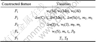
In summary, the variable set Ψ that is used for constructing new features can be determined as: Ψ= {w₀(Si), w₀(Mn), w₀(Al), Δw(C)/t_s, Δw(Mn)/t_s, Δw(Si)/t_s, m_C, m_S, Δw(S)/t_s, w₀(S), m_F, m_L, w₁(S), m_t, t_c, P_D, T₁, T_E}. The relationships among the features to be constructed and the variables in Ψ are listed in Table 1.

Table 1 Relationships among constructed features and variables

3 Improved prediction method

3.1 Feature construction based on improved GA

Feature construction [11-12] (FC) aims to transform the primitive representation of data into a new one where interactions are encapsulated into new features. If FC finds the appropriate features, such a change of representation makes the target concept easy to learn. Let  be the original feature space, and  (n is [F₁, …, F₅], and O is corresponding to the variable set Ψ. F can be expressed in the form of the product of Ψ and P () in Eq. :

where P is the parameter matrix to be optimized. According to Table 1, the parameters in P that are redundant and not used are set to zero, and the other parameters in P can be determined by GA. The optimization objective of GA is to minimize the prediction error. Fitness value can be calculated using root-mean-square error (RMSE) as

where  and  are the predict output value and real output value of sample i, respectively;  is the number of training samples.

From Table 1, it can be seen that the same variables are included in different constructed features, such as w₀(Si) and w₀(Mn) are included in F₁ and F₂, and w₁(S) is included in F₃ and F₄, which can cause high correlations among the constructed features. In the aspect of feature reduction, given the fixed input dimension, the correlation of features should be reduced to obtain more information. In order to achieve this goal, selection operation of GA is improved to reduce the correlation between coupling features. The correlation between newly constructed coupling feature vectors  and  in individual k can be evaluated by  in Eq. :

where  is the cosine value of the angle between two vectors.

The overall correlation index of individual k can be expressed as :

where C_k only contains  of coupling features, and n_k is the number of pairs of coupling features.

Roulette wheel selection method is used in GA, and the improved cumulative probability interval can be determined by

where k=1, …, n_g-1;  is the maximum value of ; n_g is the population size; α is the trade-off parameter between model accuracy and correlation of coupling features; f_I and f_A are the minimum and maximum values of fitness in current generation; C_I and C_A are the minimum and maximum overall correlation index values in current generation.

3.2 Improved ANFIS

ANFIS [13-14] combines the self-learning capability of neural networks and the fuzzy expression function of fuzzy inference system. The architecture of ANFIS used in this work for T-S model [15-16] is primarily described and shown in Fig. 2. The entire system architecture consists of five layers, namely, the fuzzy layer (L₁), product layer (L₂), normalized layer (L₃), de-fuzzy layer (L₄) and total output layer (L₅). This system has five input attributes (F₁-F₅) and one output (element yield rate).

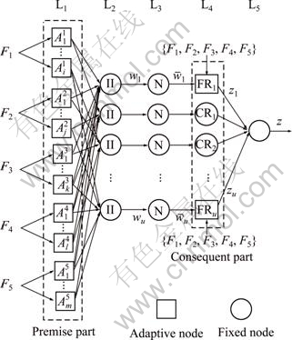
Fig. 2 ANFIS architecture

A typical fuzzy rule in Fig. 2 can be expressed as

R^p: If F₁ is  and F₂ is  and F₃ is  and F₄ is  and F₅ is

   Then z_p=F₁+F₂+F₃+F₄+F₅+

where R^p denotes the p-th rule, F₁ -F₅ are the inputs, z_p is the output attribute, (i=1, …, 6) are the consequent parameters, defined as the coefficients for the p-th rule. ,,, and  are the linguistic labels used in the fuzzy theory for dividing the membership functions (MFs).

In this work, RBF function is chosen as membership function (MF):

where c (center) and a (width) are premise parameters to determine the RBF MFs.

To avoid the limitation imposed by insufficient data samples in data-driven modeling method, empirical rules are introduced in this work. The difference between empirical rule and normal T-S rule is that the output value of empirical rule is set to be a constant value, and the value of consequent parameter and the initial values of premise parameters of empirical rules are both determined by empirical knowledge. However, the values of premise parameters are updated adaptively during learning process in order to reduce the subjectivity imposed by empirical rules. The empirical knowledge can also affect the construction of features, for the features will be constructed according to the smelting experience incorporated in empirical rules to obtain better fitness value. For example, in Fig. 2, the outputs of empirical rules (CR₁ and CR₂) are set to constant values. The outputs of the other rules (FRs) can be got through learning with samples. The improved ANFIS learning process is divided into two phases: structure identification and parameter adjustment. The detailed learning algorithm for the improved ANFIS is presented and illustrated with the system shown in Fig. 2 as follows:

1) Structure identification

It is to select the initial rules of ANFIS. To achieve this goal, firstly, smelting experience is used to determine m_r empirical rules, and convert the center parameters (c_i, i=1, …, m_r) of MFs and the crisp output values of the empirical rules into the form of input-output data pairs. Q_r is the set of converted experience dataset. Then, subtractive clustering method [17] is used to select the other system rules from training data. The aim of this clustering method is to group data by using a similarity measurement. Considering that the training dataset Q has N observations and n attributes, and Q′ is the combination of Q_r and Q, the total number of observations in Q′ is N+m_r. The density measurement at sample l is defined as

where , is the neighborhood region of attribute , which can be calculated as

In Eq. (13), K_i is an parameter larger than 2. The first selected rule is chosen as c₁ that has the largest density measurement value (D₁).

For the second rule, the effect of the first rule is subtracted in determination of the new density measurement values:

where q = l+1 and v = c_l. The data point c₂ with the largest density measurement value according to Eq. is selected out for the second fuzzy rule. The selection processes of the next rules are carried out iteratively in the same way. Let k_r be the number of selected rules. If k_r≤m_r, select the predetermined empirical rules once a time, and update the density measurement values of all the remaining data; if k_r>m_r, select the data with the largest density measurement as the next rule until the largest density measurement is not larger than zero.

2) Parameter adjustment

It is a further adjustment process for premise and consequent parameters. For the improved ANFIS, gradient descent (GD) algorithm and least square estimation (LSE) method are used for adjusting the premise parameters and consequent parameters, respectively. Premise parameter learning is to adjust a_i and c_i in the RBF MFs. The training error of sample p can be expressed as , where  is the predicted value, and  is the real value.

According to GD algorithm, the adjustment of a₁ in the system as shown in Fig. 2 can be expressed as

The adjustment of c₁ can be expressed as

where the calculations of  and  are constant values. η_a and η_c are the step-size parameters. Similarly, the adjustment of the other premise parameters is the same as the adjustment of a₁ and c₁. It can be seen that even if the consequent parts of all the fuzzy rules are  set to be constant values, the premise parameters can still be updated adaptively.

The purpose of consequent parameter learning is to adjust the consequent parameters by using LSE method. For the predetermined empirical rules, the parameters , p=1, …, m_r; therefore, the number of consequent parameters to be determined is reduced.

3.3 Implementation steps

Step 1: Set population size N_g=20, crossover rate P_C=0.6 and mutation rate P_M=0.004. The chromosome represents the parameters to be optimized in parameter matrix P. Initialize population randomly with genes that are real-coded. The value of each gene in chromosome P* is in the range of [-1, 1].

Step 2: Construct new features according to chromosome P* with all the data samples.

Step 3: Split the newly constructed data set into training set and testing set. Establish the improved ANFIS model using training set and predetermined empirical rules. Calculate the fitness value with testing set as Eq. .

Step 4: Check if the stopping criterion has been met. The stopping criterion is that the number of evolution generation is more than 200 or the RMSE value of prediction result is less than 10^-4. If yes, go to Step 6. Otherwise go to Step 5.

Step 5: Select chromosomes using the improved selection strategy, and do the crossover and mutation operation. Then, Go to Step 2.

Step 6: Stop evolution and save the optimal chromosome and the fitness value.

4 Experimental results and discussion

The study was conducted using data collected from No. 2 ladle furnace (LF) of a steel mill. 200 heats data of steel grade Q345B were collected to construct the prediction models. 180 heats were randomly selected from the dataset as training data and the others were used as testing data.

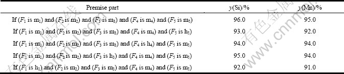
The predetermined rules that are determined by smelting experience are listed in Table 2. y(Si) and y(Mn) are yield rate values of element Si and Mn. The premise part of the smelting experiences is evaluated by fuzzy labels e.g., “medium” and “high”. More specifically, the parameters of MFs of input variable F_i correspond to “medium” (m_i) are = 1.82, = max(F_i)/2; the ones correspond to “high” (h_i) are = 1.82, = max(F_i) (i=1, …, 5).

Table 2 Empirical rules

Element yield rate models of Si and Mn are established using the proposed method. In the selection operation, set α=0 and α=0.2 in Eq. of each model, respectively. α=0 means that C_k is not included in the selection operation. The relationships between the best fitness values and the evolution of different values of α are shown in Fig. 3. It is noted that the improved GA (α=0.2) takes 87 and 104 generations for yield rate predictions of Si and Mn to reach the optimal solutions, while the original GA (α=0) takes 148 and 152 generations for yield rate predictions of Si and Mn to reach the near-optimal solutions. The optimal solutions of improved GA are 0.65×10^-2 and 0.52×10^-2 for Si and Mn, which are better than the near-optimal solutions of original GA with 0.96×10^-2 and 0.88×10^-2 for Si and Mn. It is shown that because of the joining of correlation index of coupling features in the selection process, the convergence rate is speeded up and the local optima can be avoided effectively.

The features constructed using improved GA with α=0.2 are listed in Table 3, and the numbers of ANFIS rules are 25 and 27 for Si and Mn yield rate models, respectively.

The proposed method (Method 1) is compared with the combination method of original GA and improved ANFIS (Method 2), the combination method of original GA and original ANFIS (Method 3), reference heats method in Ref. [1], and BP neural network in Ref. [2]. For BP method, the input variable set is Ψ. Prediction results of these methods are shown in Fig. 4. RMSE and maximum absolute error (MAE) of the results of these methods are listed in Table 4.

It can be seen that the prediction accuracy of the proposed method is better than the other methods. For both Si and Mn, the accuracy of the proposed method is better than Method 2. It is also revealed that the improved selection operation in GA plays an important role to avoid the search being trapped in local optima. The accuracy of Method 2 is better than Method 3, which justifies the incorporation method of smelting experiences, since, incorporated with smelting experiences, it deals successfully with the uncertainty and subjectivity associated with human performance assessment, and alleviates the shortage of data-driven method effectively.

The proposed method has been practically tested with 780 heats of Q345B in manufacturing processes in a steel mill. The testing results are shown in Fig. 5. The  hit rates of Si and Mn yield rate predictions after using the proposed method reach 98.08% and 98.21% in error range of ±1%, respectively, compared with 81.79% and 83.21% before using the proposed method. It is   shown that the hit rates of element yield rates can increase remarkably. With the increase of element yield rate, the time of secondary alloying process and the usage of alloy materials can be reduced.

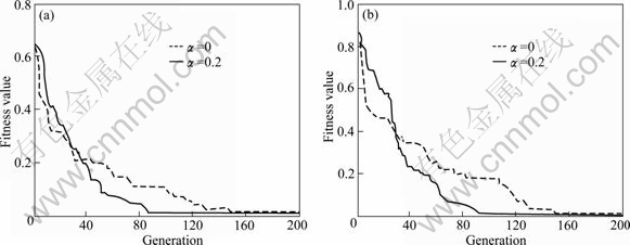
Fig. 3 Optimization processes with different α: (a) Best fitness values of Si; (b) Best fitness values of Mn

Table 3 Constructed features of Si and Mn yield rate prediction models

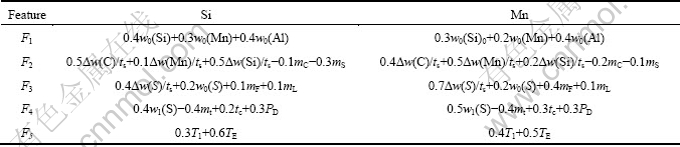
Table 4 Comparisons of prediction results of different methods (10^-2)

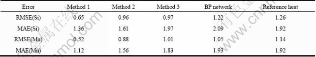
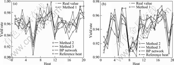
Fig. 4 Comparisons of element yield rate predictions: (a) Si; (b) Mn

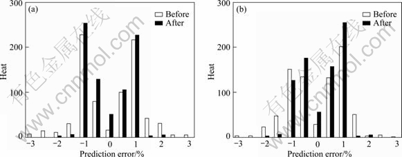
Fig. 5 Histogram of element yield rate prediction errors: (a) Prediction errors of Si; (b) Prediction errors of Mn

5 Conclusions

1) The feature construction method based on improved GA paves the way for incorporating human experience into ANFIS, and the improved selection operation in GA can effectively speed up the convergence rate and reduce the chance of being trapped in local minima.

2) The improved ANIFS method that combines the smelting experience and the training data solves the shortage of data-driven modeling method, and improves the accuracy of the element yield rate prediction.

3) Both the experimental and testing results reveal that compared to the other prediction methods, the proposed approach has excellent prediction accuracy and the fast prediction speed.

4) Because calculation speed is increased by using proposed method, accuracy of predicted element yield rate can satisfy refining requirements, and the refining cycle and cost of production effectively can be reduced.

References

[1] YU Peng, ZHAN Dong-ping, JIANG Zhou-hua, LI Da-liang, YIN Xiao-dong, MA Zhi-gang. Development of a terminal composition prediction model for steel refine with ladle furnace [J]. Journal of Materials and Metallurgy, 2006, 5(1): 20-22. (in Chinese)

[2] NATH N K, MANDAL K, SINGH A K. Ladle furnace on-line reckoner for prediction and control of steel temperature and composition [J]. Ironmaking and Steelmaking, 2006, 33(2): 140-150.

[3] GAO Xian-wen, ZHANG Ao-an, WEI Qing-lai. Neural network based prediction of endpoint in ladle refining process [J]. Journal of Northeastern University: Natural Science, 2005, 26(8): 726-728. (in Chinese)

[4] HU Q H, CHE X J, ZHANG L, YU D R. Feature evaluation and selection based on neighborhood soft margin [J]. Neurocomputing, 2010, 73(10/11/12): 2114-2124.

[5] TEIXEIRA R, TOME M, LANG W. Unsupervised feature extraction via kernel subspace techniques [J]. Neurocomputing, 2011, 74(5): 820-830.

[6] DING M T, TIAN Z, XU H X. Adaptive kernel principal component analysis [J]. Signal Processing, 2010, 90(5): 1542-1553.

[7] HWANG S F, HE R S. Improving real-parameter genetic algorithm with simulated annealing for engineering problems [J]. Advances in Engineering Software, 2006, 37(6): 406-418.

[8] MCCALL J. Genetic algorithms for modelling and optimization [J]. Journal of Computational and Applied Mathematics, 2005, 184(1): 205-222.

[9] YU Shou-yi, KUANG Su-qiong. Fuzzy adaptive genetic algorithm based on auto-regulating fuzzy rules [J]. Journal of Central South University of Technology, 2010, 17(1): 123-128.

[10] LI Jing. LF refining technology [M]. Beijing: Metallurgical Industry Press, 2009: 121-125. (in Chinese)

[11] HAFTI S, PEREZ E. Evolutionary multi-feature construction for data reduction: A case study [J]. Applied Soft Computing, 2009, 9(4): 1296-1303.

[12] AVRILIS D, TSOULOS G, DERMATAS E. Selecting and constructing features using grammatical evolution [J]. Pattern Recognition Letters, 2008, 29(9): 1358-1365.

[13] JANG R. ANFIS: adaptive-network-based fuzzy inference system [J]. Systems, Man and Cybernetics, IEEE Transactions on, 1993, 23(3): 665-685.

[14] SHOOREHDELI M A, TESHNEHLAB M, SEDIGH A K, KHANESAR M A. Identification using ANFIS with intelligent hybrid stable learning algorithm approaches and stability analysis of training methods [J]. Applied Soft Computing, 2009, 9(2): 833-850.

[15] TAKAGI T, SUGENO M. Fuzzy identification of systems and its applications to modeling and control [J]. Systems, Man and Cybernetics, IEEE Transactions on, 1985, 15(1): 116-132.

[16] SU Cheng-li, LI Ping. Adaptive predictive functional control based on Takagi-Sugeno model and its application to pH process [J]. Journal of Central South University of Technology, 2010, 17(2): 363-371.

[17] EFTEKHARI M. Extracting compact fuzzy rules for nonlinear system modeling using subtractive clustering, GA and unscented filter [J]. Applied Mathematical Modelling, 2008, 32(12): 2634-2651.

(Edited by YANG Bing)

Foundation item: Projects(2007AA041401, 2007AA04Z194) supported by the National High Technology Research and Development Program of China

Received date: 2011-08-11; Accepted date: 2012-01-05

Corresponding author: XU Zhe, PhD Candidate; Tel: +86-18624038570; E-mail: xuzhe83@gmail.com