Numerical simulation of mold-temperature-control solidification

YOU Dong-dong(游东东), SHAO Ming(邵 明), LI Yuan-yuan(李元元), ZHOU Zhao-yao(周照耀)

Department of Mechanical Engineering, South China University of Technology, Guangzhou 510640, China

Received 20 October 2006; accepted 25 December 2006

Abstract: A finite element method(FEM) for the numerical simulation of the columnar part of the mould-temperature-control solidification(MTCS) process was presented. The latent heat was taken into account and 3D transient heat transfer analysis was carried out by using the developed FEM software. The relative errors between the numerical and experimental data are less than 6%. Three MTCS cases were computed with this method. The first case only opens the cooling channels in the bottom of the mold. The second case individually controls the separate 7 groups of cooling channels by giving 7 control points. When the temperature of a control point reaches the preset value of 400℃, the corresponding channel will be opened. The third case opens all the cooling channels at the same time. The results indicate that in the second case, the solid-liquid interface keeps near-planar. The growth velocity of the solid-liquid interface is 0.3-0.4 mm/s, which is greater than 0.1-0.3 mm/s of the first case, performing better than the others. Thus the forming quality and efficiency part interior can be improved by mold-temperature-control and the numerical model is validated. The numerical simulation of MTCS can provide an available tool for the advanced investigation on the defect improvement and the crystal’s quality.

Key words: mold-temperature-control solidification; columnar part; numerical simulation; solid-liquid interface

1 Introduction

In heat processes, such as solidification process, mold temperature, is an important factor to improve the forming quality by influencing melt temperature, viscosity, pourability and setting time, etc[1-5]. Mold- temperature-control forming uses artificial intelligence method to control the mold temperature based on the real-time state during the whole forming process so as to improve the quality of the workpiece[4-6].

Both the liquid and solid phase temperature of the workpiece in the mold-temperature-control solidification (MTCS) process must be obtained accurately to research the relationship of the forming state and control parameters for mold temperature[7-11]. In this paper, a FEM method for the numerical simulation of the MTCS process of the columnar part was presented[12-18]. The latent heat was taken into account and the 3D transient heat transfer analysis was carried out. The numerical simulation of MTCS cases can provide a tool for the advanced investigation of MTCS technology and knowledge towards intelligent control.

Fig.1 illustrates the MTCS process of the columnar part. Many individual temperature control units including heating units, cooling units and adiabatic units are equispaced in the mold. The melt is poured into the mold that is preheated, then, the cooling units in the bottom of the mold are opened. In the solidification process, automatic control equipment obtains the real-time temperature data from the thermocouples and controls the mold temperature field by adjusting the individual temperature control units in the side of the mold. The heat-transfer process is very complicated in MTCS, so the physical model is simplified as follows:

1) Ignore the convection in the melt;

2) Ignore the mass transfer in the liquid and solid materials;

3) At the beginning of the solidification, the tem- perature distribution of the mold and melt is uniform respectively.

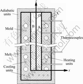
Fig.1 MTCS process of columnar part

3 Mathematical model

3.1 Heat transfer equation

The finite element method was adopted to compute the temperature field and the simplified one-fourth model was computed for symmetry. Fig.1 shows the simulation coordinates, where the grid origin is at the geometric centre of the contact face between the bottom of the workpiece and the mold. The positive direction of z axis follows the solidification direction. The transient heat transfer equation in the MTCS process is

where  T is the transient temperature of a certain point in the model, λ is the conductivity, ρ is the density, c is the specific heat capacity, t is the time, and  is the heat source from heating units or latent heat. In case of latent heat,  can be expressed as

where  L is the latent heat and f_s is the mass fraction of solid when the temperature is T. The latent heat can be computed by the temperature compensation method[3]. As to the initial steady process, the heat transfer equation is

3.2 Boundary conditions

The boundaries A-D shown in Fig.1 were processed as follows:

1) Boundary A: convection between the melt surface and air in the mold cavity and radiation between the melt surface and mold are ignored.

2) Boundary B: contact faces between the work- piece and mold are treated as an ideal contact.

3) Boundary C: contact faces between the adiabatic units and mold are treated as an ideal adiabatic boundary.

4) Boundary D: either ?T/?y=0 or ?T/?x=0 exists in the symmetry plane.

3.3 Processing of mold temperature control units

1) Heating units are considered as heat sources.

2) Adiabatic units are handled as boundary condi- tions, instead of as computational objects.

3) Cooling units are processed in terms of the forced convection of the coolant in channels. Heat convection in the coolant flow can be expressed as follows:

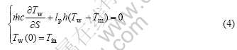
where   is the mass flow rate, c is the specific heat capacity, T_w(t) is the coolant temperature, T_m(t) is the mold temperature, S is the streamline coordinate, l_p is the perimeter of channel section, h is the force convection heat transfer coefficient, and T_in is the inlet initial temperature.

In solidification process, the heating units and cooling channels are controlled by means of the temperature at appointed spots. In numerical simulation, the usual processing for the mold temperature control units is to assume their working duration or time increment steps. For heating units, heat sources are defined by the function of time as the formula  For cooling units, in given time steps heat transfer is computed according to Eqn.(4). In this paper, the method was different and closer to the practical process. A mold temperature control units module was developed. In the module, every unit is initially given a corresponding control node. During a certain time step, the temperature of the control node(s) reaches the critical value for switching the units, the module is signaled to compute the changed state for the next step.

4 Numerical method and programming

Equivalent integral formulae and FEM equations of the before-mentioned differential equations and boundary conditions were established with the Galerkin weighted residual method. The discrete time domain was processed with the receding difference method that is unconditionally stable. The final linear algebraic system was solved using the conjugate gradient iterative method with preconditioning.

Fig.2 shows the architecture of the MTCS software. Pre and post processing work use MSC.marc software. The solver is divided into 10 modules, where 9 modules have the specific functions as shown in Fig.2 and the 10th is the common data processing module. The Fortran codes take up more than 5 000 lines. The system and individual modules were tested normal in many aspects, such as the accuracy of the results, computational efficiency, system reliability and error solution.

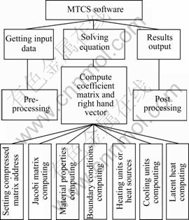
Fig.2 Numerical simulation software of MTCS

5 Analysis of computed cases

5.1 Experimental verification of numerical simulation

5.1.1 Simulation condition

The forming columnar part was 270 mm×45 mm×45 mm. The mold wall was 40 mm in thickness and 450 mm in height. 6 channels of 5 mm diameter were machined in the mold bottom and 7 pairs of channels and 8 pairs of heat pipes were equispaced 50 mm apart in the mold sides. The mold material was chrome steel whose density was 7 850 kg/m³. The workpiece material was pure Zn whose latent heat capacity was 1.13×10⁵ J/kg and whose solid-liquid phase critical temperatures are 417.45℃ and 419.45℃ respectively. The other properties are given in Fig.3. The simplified one-fourth model was computed for symmetry. The computational mesh is shown in Fig.4, where the dark part is the workpiece; the gray part is the mold. The model was divided into 3876 8-node hexahedron elements including 5 393 nodes. The element size is about 6 mm. The process was as follows: after preheating to 470 ℃, the mold was filled with Zn melt of 450 ℃. The heating units were closed and the channels in the bottom were opened until the solidification was complete. The cooling water has an initial temperature of 20 ℃, a mass flow rate of 0.017 kg/s, and a convection heat transfer coefficient of 1 300.

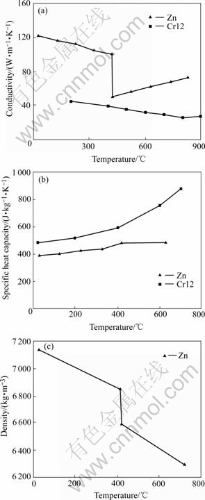
Fig.3 Properties of materials

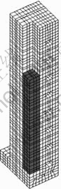
Fig.4 Computational mesh division

5.1.2 Experiment conditions

Experiment device includes the mold and tempera- ture measure and control system. Channels were machined in the mold connecting with outer copper pipes. The mold wrapped with adiabatic materials can be heated by far infrared pipes. The control system, which involves a P4 computer, a temperature collection module and an output control module, switches the far infrared pipes or electromagnet valves installed on copper pipes by relays. All the process data were operated by MCGS configuration software.

5.1.3 Comparison of experimental and numerical data

Fig.5 shows the cooling curves of five points down the centre line of one side of the workpiece. They lie at z=25, 75, 125, 175 and 225 mm, respectively. These points were numbered in z coordinate sequence with the letter e or n following the numbers meaning experimental or numerical results respectively. The relative errors in the two groups of data are less than 6% as reckoned from model assumption, experimental measuring error and material properties data.  Thereby, the numerical model is valid.

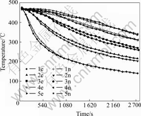
Fig.5 Comparison of experimental and numerical data

5.2 Analysis of three modification in forming cases

5.2.1 Introduction of three cases

Three modifications were simulated using the numerical model of section 5.1 as the control.

Case 1: open the bottom channels only. The other conditions are same as section 5.1.

Case 2: control the seven pairs of side channels individually. The initial conditions are same as case 1. In solidification process, seven temperature control points located down the center line of one side of the workpiece monitor the corresponding channels which are 10 mm above the points. They lie at z=25, 75, 125, 175, 225, 275 and 325 mm, respectively, and their numbers and other appointments reference section 5.1.3. When the temperature of a control point reaches the preset value of 400 ℃, the corresponding channel will be opened.

Case 3: open all channels at the beginning of the process until solidification is complete. The initial conditions are the same as case 1.

5.2.2 Results analysis and discussion

The computed temperature fields of the three cases are shown in Fig.6, where the five graphs in Fig.6(a) show the temperature isosurfaces of t=180, 450, 720,1 170 and 1 620 s in case 1. The five graphs in Fig.6(b) show the temperature isosurfaces of t=90, 180, 360, 540 and 720 s in case 2. Finally, the five graphs in Fig.6(c) show the temperature isosurfaces of t=100, 150, 200, 250 and 300 s in case 3. The solidification was complete in 1 800 s in case 1, 800 s in case 2 and 150 s in case 3.

In case 3, although the cooling was faster than the other two cases, the temperature isosurfaces were irregular and move from the channels in the bottom and sides to upper center of the workpiece. Accordingly, the solidification occurred from the sides and bottom to the upper center of the workpiece. Acted on by solidification shrinkage and the gravity, the melt of the upper center will feed downward and it tends to form shrinkage cavity in this part. Because of maintaining planar temperature isosurfaces in case 1, the solid-liquid interface moved up along the z direction as the solidification progressed. This is considered directional solidification and its velocity dropped gradually from the initial approximately 0.3 mm/s to 0.1-0.15 mm/s as the solid-liquid interfaces move away from the bottom channel. Compared with case 1, the near-planar temperature isosurfaces of case 2 are little accidented. It still considered directional solidification but its velocity remained at about 0.3-0.4 mm/s. In solidification process, the side channels will be opened from bottom to top. When the temperature of a control point reaches the preset value of 400 ℃, the melt under the point will solidify. Then the corresponding channel will be opened. Resultingly, the mold and solid metal will be cooled faster and the crystalline growth velocity of the upper melt will be promoted. Therefore, the solidification velocity may not descend like case 1.

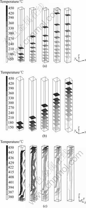
Fig.6 Computational temperature fields of three cases: (a) Case 1; (b) Case 2; (c) Case 3

Unlike case 3, the planar or near-planar solid-liquid interfaces of cases 1 and 2 are propitious to improve the crystal quality and obtain columnar crystals of directional growth. This is especially true in case 2, since the solidification velocity, which is about twice of case 1, can be increased by adjusting the channel’s parameters and the temperature isosurfaces keep near-planar. Accordingly, case 2 is shown to be better than the others and it is seen that the forming quality can be improved by mold temperature control.

6 Conclusions

1) Physical and mathematical models of the MTCS temperature field were established. The computational software was developed to simulate the forming process of the columnar part. The validity of the numerical model was proved by comparing the computational with experimental data.

2) The computational temperature fields of three cases indicate that the 2nd case that controls the mold temperature by cooling channels in the mold sides is better than the others. Hence, mold temperature control forming technology is seen to help to improve the forming quality.

References

[1] TAO Yu-lan. The influence of mold temperature on die-casting part quality [J]. Special Casting and Nonferrous Alloys, 1995(1): 23-30. (in Chinese)

[2] LI Yuan-yuan, XU Zhen, NI Dong-hui. Review of heating system in warm compaction equipment [J]. Powder Metallurgy Industry, 2000, 10(6): 14-18. (in Chinese)

[3] XIONG Shou-mei, XU Qing-yan, KANG Jin-wu. The Simulation Technology of Casting Process [M]. Beijing: China Machine Press, 2004.

[4] FERNANDO C C, LAN C, CHRIS P. Mould temperature control in continuous casting for the reduction of surface defects [J]. ISIJ International, 2004, 44(8): 1393-1402.

[5] YU Yan-dong, JIANG Hai-yan, LEI Li, ZENG Xiao-qin, ZHAI Chun-quan, DING Wen-jiang. Numerical simulation of die casting process of magnesium alloy [J]. Journal of Central South University: Science and Technology, 2006, 37(5): 867-873. (in Chinese)

[6] HSIEH S S. Transient analysis of the waterlines effect in the die casting dies [J]. Applied Mathematical Modeling, 1998, 13(5): 282-290.

[7] SI H, CHO C, KWAHK S. A hybrid method for casting process simulation by combing FDM and FEM with an efficient data conversion algorithm [J]. Journal of Materials Processing Technology, 2003, 133(3): 311-321.

[8] FENG Jian, ZHANG Chang-rui, HUANG Wei-dong. Numerical simulation on near-rapid directional solidification process of Al bar sample [J]. The Chinese Journal of Nonferrous Metals, 2004, 14(3): 329-334. (in Chinese)

[9] DAVEY K, BOUNDS S. Modeling the pressure die casting process using boundary and finite element methods [J]. J Mater Process Technol, 1996, 63(123): 696-700.

[10] LEE Y C, LEE S M, CHANG Q M, CHOI J K, HONG C P. Modeling of mold filling and solidification sequence in the permanent mold casting process with an automated water cooling system [C]// THOMAS B G, BECKERMANN C. Proceeding of International Conference on Modeling of Casting, Welding and Advanced Solidification Process VIII. San Diego: The Minerals, Metals and Materials Society, USA, 1998: 85-92.

[11] XUE Xiang, ZHOU Bi-de, ZHANG Yue-bing, XIAO Jin. Numerical simulation of mold filling and solidification process of an h-shape steel billet in water cooling permanent mold [J]. Foundry, 2003, 52(12): 1182-1185. (in Chinese)

[12] GUO Ge, QIAO Jun-fei, WANG Wei. Simulation of slab solidification with computer [J]. The Chinese Journal of Nonferrous Metals, 1999, 9(2): 339-344. (in Chinese)

[13] LI Zhao-xia, ZHENG Xian-shu, JIN Jun-ze. Determination of heat transfer coefficient in continuous casting [J]. Foundry, 2001, 50(1): 141-144. (in Chinese)

[14] PEHLKE R D, BERRY J T. Heat transfer at the mold/metal interface in permanent mold casting of light alloys [C]// Conference Proceedings from Materials Solutions 2002: Advances in Aluminum Casting TechnologyⅡ. Columbus, OH, USA, 2002: 177-184.

[15] MORAN G J, BOUNDS S M, PERICLEOUS K A, CROSS M. Prediction of cold shuts using an unstructured mesh finite volume code [C]// THOMAS B G, BECKERMANN C. Proceedings of International Conference on Modeling of Casting, Welding and Advanced Solidification Process VIII. San Diego: The Minerals, Metals and Materials Society, USA, 1998: 101-108.

[16] SUN Xiao-bo, ZHANG Chun-hui, WANG Xi-jun, AN Ge-yin, ZHAO Guo-qi, LIU Xin-zhong, LU Min, NING Ru-yi. Numerical simulation of solidification process and experimental verification of precision casting of al alloy in gprsum mold [J]. The Chinese Journal of Nonferrous Metals, 1998, 8(4): 631-636. (in Chinese)

[17] HOU Hua, CHENG Jun, XU Hong. Development of CAD softwave package of intellectualized casting technology [J]. Journal of Central South University of Technology: English Edition, 2005, 12(3): 280-283.

[18] HU Han-qi, SHEN Ning-fu, YAO Shan, WANG Zi-dong. Principle of Metal Solidification (2nd ed) [M]. Beijing: China Machine Press, 2000.

Corresponding author: YOU Dong-dong; Tel: +86-20-87112973; E-mail: youdd@sina.com

(Edited by YANG Hua)