J. Cent. South Univ. (2012) 19: 944-952

DOI: 10.1007/s11771-012-1096-0

Numerical computation and analysis of unsteady viscous flow around autonomous underwater vehicle with propellers based on sliding mesh

GAO Fu-dong(高富东)¹, PAN Cun-yun(潘存云)¹, HAN Yan-yan(韩艳艳)²

1. College of Mechatronic Engineering and Automation, National University of Defense Technology,Changsha 410073, China;

2. SANY Heavy Industry Co., Ltd., Changsha 410100, China

? Central South University Press and Springer-Verlag Berlin Heidelberg 2012

Abstract: The flexible transmission shaft and wheel propeller are combined as the kinetic source equipment, which realizes the multi-motion modes of the autonomous underwater vehicle (AUV) such as vectored thruster and wheeled movement. In order to study the interactional principle between the hull and the wheel propellers while the AUV navigating in water, the computational fluid dynamics (CFD) method is used to simulate numerically the unsteady viscous flow around AUV with propellers by using the Reynolds-averaged Navier-Stokes (RANS) equations, shear-stress transport (SST) k-w model and pressure with splitting of operators (PISO) algorithm based on sliding mesh. The hydrodynamic parameters of AUV with propellers such as resistance, pressure and velocity are got, which reflect well the real ambient flow field of AUV with propellers. Then, the semi-implicit method for pressure-linked equations (SIMPLE) algorithm is used to compute the steady viscous flow field of AUV hull and propellers, respectively. The computational results agree well with the experimental data, which shows that the numerical method has good accuracy in the prediction of hydrodynamic performance. The interaction between AUV hull and wheel propellers is predicted qualitatively and quantitatively by comparing the hydrodynamic parameters such as resistance, pressure and velocity with those from integral computation and partial computation of the viscous flow around AUV with propellers, which provides an effective reference to the study on noise and vibration of AUV hull and propellers in real environment. It also provides technical support for the design of new AUVs.

Key words: computational fluid dynamics; sliding mesh; wheel propeller; autonomous underwater vehicle; viscous flow field

1 Introduction

The autonomous underwater vehicles (AUVs) are promising for navy use because they can fulfill many missions such as assaults, communications and obviating torpedoes. The multi-moving state of AUV in this work makes use of the flexible transmission shaft based on spherical gear as the kinetic source equipment, on the end of which a new wheel propeller is installed [1]. The whole equipment can achieve four functions such as wheels, legs, thrusters and course control based on the characteristics of spatial deflexion and continual circumgyratetion of the flexible transmission shaft. The rudders and vectored thrusters are used to control the course at high speed and low speed, respectively. The typical motions of AUV are shown in Fig. 1 [2]. The pumping action of four wheel propellers changes the pressure distribution and boundary layer thickness of AUV hull, while the uneven wake of AUV hull changes the inlet condition of wheel propellers, which results in unsteady and uneven load distribution and causes the cavitation, noise and vibration. Therefore, the viscous flow of AUV with propellers is very complicated and the interaction between AUV hull and propellers is concerned by designers, which has important theoretical and practical significance.

Nowadays, there are two main methods used to study the interaction between AUV hull and propellers including model experiment and numerical computation. Model experiment is mainly composed of self-propulsion test and nominal wake field test. Experimental data can be used to get some average amount of the interaction between AUV hull and propellers, such as wake fraction and thrust deduction. The study of interactional principle gets some progresses through the non-contact measurement around the flow field with laser doppler velocimetry (LDV) and particle image velocimetry (PIV) experimental techniques. But the model experiment needs high cost and long cycle, which is also influenced by scale effect and environmental interference. So, it is difficult to reflect intuitively and accurately the real situation of the flow field [3]. Numerical computation that uses the potential theory and boundary layer cannot accurately simulate the interaction between AUV hull and propellers early because the flow is assumed to be irrotational and the viscous effect is neglected [4]. With the Reynolds-averaged Navier-Stokes (RANS) equations used to solve flow field, the computational precision is improved, which provides technical support for the study of the interaction between AUV hull and propellers. But, it is difficult to compute the integral flow field because of the complicated geometry and the interaction between AUV hull and propellers. Nowadays, force field simulation is usually applied to studying the interaction, which couples the computation program of AUV hull and the open-water performance prediction program of propellers through volume force [5-6]. But, the computation is only a rough approximation because only the thrust of propeller, not the complicated geometry, is taken into account by the volume force instead of the real propeller. As the capability of computers has greatly advanced, it is possible to introduce computational fluid dynamics to compute the integral flow field of AUV with propellers. The numerical computation of the integral flow field introduces mainly mixed-surface method and sliding mesh approach. The mixed-surface method simulates the mutual interaction of the rotary and static computational domains based on mixed-surface model. It is an approximate method because the two computational domains are solved as a steady problem and all hydrodynamic parameters at the interface are passed after circumferential average [7]. The sub-domains hybrid mesh that adapts to the integral calculation of the viscous flow around AUV with propellers is designed according to its geometry and flow field. Then, CFD method is used to simulate numerically the unsteady viscous flow around AUV with propellers by using the RANS equations and shear-stress transport (SST) k-w model based on sliding mesh, which provides an accurate and practical numerical method for the study of the interaction principle and the design of new AUVs.

2 Mathematical modeling

2.1 Governing equation and boundary condition

The main geometrical parameters of the AUV with propellers are listed in Tables 1 and 2. The wheel propeller is a thruster designed according to its movement needs. The water is assumed to be incompressible and isothermal Newtonian fluid. The governing equations are written for the mass and momentum conservation as

                                                       (1)

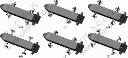
Fig. 1 Typical motions of AUV with propellers: (a) Cruising forward; (b) Vertical descend; (c) Transverse turning; (d) Wheeled moving or transverse pushing; (e) Landing sea-bottom or vertical ascending; (f) Pivot steering or crawling on sea-bottom

Table 1 Geometrical parameters of AUV

Table 2 Geometrical parameters of wheel propeller

              (2)

where ρ is the density, t is the time, u_i and u_j are the

velocities in Cartesian coordinate system,  is the Reynolds stress, μ is the molecular viscosity, p is the static pressure, f_i is the unit mass force and δ_ij is the Kronecker delta.

The SST k-w turbulence model is used for turbulence closure, which is the sum of the standard k-ε model and the standard k-w model multiplied by a mixed function, respectively. So, it combines the advantages of the standard k-w model computing near the wall and the standard k-ε model computing in the far field [8]. The SST k-w model has different turbulence constants, which not only increases a horizontal dissipation derivative but also takes into account the transport process of turbulent shear stress in the definition of turbulent viscosity compared with the standard k-w model. These features make the SST k-w model have a wider applicable scope and greater computational accuracy. According to the Boussinesq’s assumption, The SST k-w turbulence model can be written in Cartesian tensor form as

   (3)

where k is the turbulence kinetic energy, w is the specific dissipation rate, Γ_k is the effective diffusivity of k, Γ_w is the effective diffusivity of w, G_k is the generation of k due to mean velocity gradients, G_w is the generation of w due to mean velocity gradients, Y_k is the dissipation of k due to turbulence, Y_w is the dissipation of w due to turbulence, and D_w is the cross-diffusion term.

The specific expressions above are written as

                  (4)

where σ_k is turbulent Prandtl number for k; σ_w is the turbulent Prandtl number for w; μ_t is the turbulent viscosity; S is the strain rate magnitude; F₁ is the blending function; β^*, β_i and σ_w,2 are all constants.

The boundary conditions of computational domain include inlet, outlet, wall, outside and symmetry plane, as shown in Fig. 2, the specific settings are as follows (L is the length of AUV).

1) On the inlet boundary 0.5L away from the AUV’s head, velocity components of uniform stream with the given inflow speeds are imposed.

2) On the exit boundary 1.0L away from the AUV’s stern, static pressure is set to be zero while other variables are extrapolated.

3) On the AUV’s surface, the non-slip condition is imposed.

4) On the outer boundary 0.6L away from AUV’s side surface, the velocity components are given to avoid the flow field affected by the computational domain size.

5) On the extended surface of the longitudinal symmetry plane, the symmetry condition is imposed to reduce by half the amount of computation.

The definition of the coordinate axes is that x axis points to downstream, y axis points to starboard and z axis accords with right hand principle. The coordinate origin is the intersection of upside surface, the longitudinal symmetry plane and the cross-section of head.

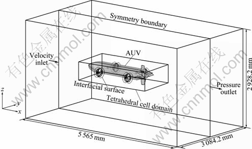
Fig. 2 Computational domain of integral flow field around AUV with propellers

2.2 Mesh generation and numerical method

The quality of grid directly determines the convergence, efficiency and accuracy of computation. Therefore, a reasonable mesh should be generated based on the physical characteristics of the flow field. The computational domain is divided into three regions according to AUV’s geometry, where the size function is used to control mesh density. Two cylinders are founded as the computational domains of two wheel propellers, respectively, where a revolving coordinate system is fixed on each wheel propeller and tetrahedral cells are filled. Then, a cuboid which contains two small cylinders is founded to enclosure AUV hull and tetrahedral cells are filled. The remaining flow fields outside are filled with hexahedral cells and a static coordinate system is found for computation. The sub-domain hybrid mesh not only adjusts the complicated shape of AUV with propellers, but also improves the mesh precision and reduces the number. The surface mesh of the AUV with propellers is shown in Fig. 3.

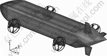
Fig. 3 Surface mesh of AUV with propellers

Sliding mesh is used to transfer data between the computational domains of AUV hull and wheel propellers. In order to achieve mutual sliding, the mesh nodes on both interfacial sides are not required to overlap. The data can be transferred through computing the fluxes in coincident section of the interfacial sides at each time step, as shown in Fig. 4. The interfacial domain comprises several surfaces such as A-B, B-C, D-E and E-F, which generate interfacial surface composed by a-b, b-c and c-d, and among them, b-c, c-d and d-e compose the internal regions, as shown in Fig. 5. In order to compute the fluxes that flow into unit III, unit I and unit II send information to unit III through surfaces b-c and c-d instead of D-E.

The mathematics model of flow field is a series of nonlinear equations, which employs a cell-centered finite volume method that allows the adoption of computational elements with arbitrary polyhedral shape. Convection terms are discretized using a second-order accurate upwind scheme, while diffusion terms are discretized using a second-order accurate central differencing scheme. The velocity-pressure coupling and overall solution procedure are based on a PISO (pressure impact with splitting of operations) type segregated algorithm. The time step of the computation is 0.002 s and 50 times of iteration is carried out at each time step. The convergence criterion is set as 0.000 1.

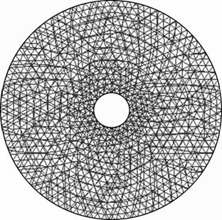
Fig. 4 Sliding mesh of interfacial domain

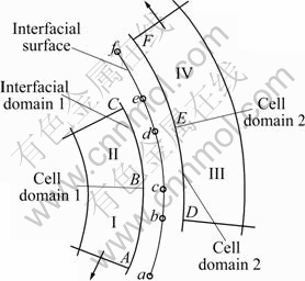
Fig. 5 Principle of data transfer between stationary mesh and sliding mesh

3 Hydrodynamic performance of AUV hull and wheel propeller

In order to study the interactional principle between AUV hull and wheel propellers and validate the correctness of the numerical method, the numerical simulation of steady viscous flow around AUV hull and propellers, namely partial computation, is carried out by using the RANS equations, SST k-w model and SIMPLE algorithm before the integral computation of viscous flow around the AUV with propellers.

3.1 Numerical computation of open-water performance of wheel propeller

The wheel propeller is designed based on the D4-70 propeller in China Ship Scientific Research Centre (CSSRC), which has dual functions of wheels and thrusters with high strength characteristics and good open-water performance [9].

Inflow speed is given to the inlet of the computational domain 4D away from the propeller upstream. Static pressure is given to the outlet 6D away from the propeller downstream. Sliding wall is given to the outer boundary 4D away from the hub axis [10-11]. The cylinder that contains the propeller is filled with tetrahedral cells, and the other domain beyond is filled with hexahedral cells. The number of total cells is    852 357.

The rotation speed of propeller is 10 r/s and the advance ratios vary from 0.1 to 1.1, which are achieved through varying the inflow speed. The comparison between computational data and experimental data of the open-water performance of D4-70 propeller is listed in Table 3, which indicates that the computational values are in good agreement with the experimental data. The maximum error value between the computational K_t (thrust coefficient) and K_q (corque coefficient) with varying advance ratios and that of experimental data is 5.93%. The errors between the computational data and experimental data increase gradually while J >0.8, and the maximum error is 6.24%, which is mainly due to the reverse error of K_t and K_q. The numerical computation method is verified by the good precision, which proves that this method fits to design propellers [12-13].

The open-water performance of the wheel propeller at positive and reversing rotation state is shown in Fig. 6. Compared with the computational results of propeller D4-70, the thrust performance is improved when 0.1≤J≤0.8, while K_q with varying advance ratios increases slightly, which causes the open-water efficiency of the wheel propeller to decrease. But the wheel function with high strength of the wheel propeller is realized and its maximum allowable load is 3 975 N [14-15]. As a whole, the wheel propeller has the characteristics of high thrust, high structural strength, stable hydrodynamic performance and anti-blade flutter, which can meet the design requirements of AUVs propellers.

3.2 Numerical computation of hydrodynamic characteristics of AUV hull

The AUV hull in this work adopts NPS II AUV’s figure. The mesh of AUV hull generates through replacing two wheel propellers for tetrahedral cells based on the mesh of AUV with propellers and they have the same boundary conditions.

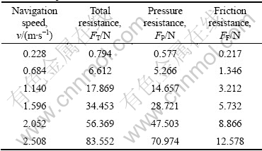
The flow is sluggish in the front of the AUV’s head and accelerated at its both sides due to the high block coefficient. So, the high-pressure zone is formed in the front and the ??low-pressure zone is formed at the both sides. The large low-pressure area is formed due to the shape of four flexible transmission shafts, which increases pressure resistance. Figure 7 shows the relative pressure intensity distribution of AUV hull navigating at 1.14 m/s. Table 4 gives computational results of the resistance of AUV hull, which can be seen that 72.7% of the total resistance is pressure resistance, while the proportion of friction resistance is very small.

Table 3 Comparison of open-water performance of D4-70 propeller between computational data and experimental data

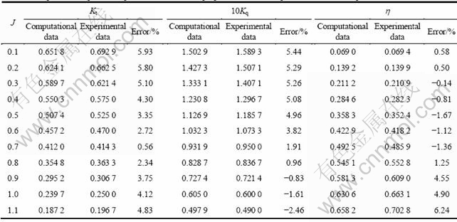
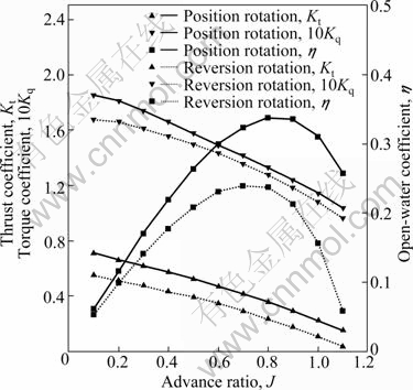
Fig. 6 Open-water performance of wheel propeller at positive and reversing rotation states

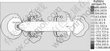
Fig. 7 Relative pressure intensity distribution of AUV hull in horizontal plane (Y/L=-0.079 5)

Table 4 Computational resistance of AUV hull

4 Hydrodynamic characteristics of AUV hull with propellers

The AUV with propellers has four wheel propellers. In this work, the interaction of AUV hull and wheel propellers is studied in the cruise mode where flexible shafts point to the stern. When the rotation speeds of wheel propellers are all 10 r/s, the integral flow field of AUV hull with propellers is computed numerically at different speeds based on sliding mesh.

The resistance coefficients of AUV hull and wheel propellers (C_d1, C_d2, and C_d3) with varying times are periodic at the speed of 1.14 m/s, which are got by time step mode, as shown in Figs. 8 and 9. The computational results achieve stability from 9.0 s. Due to the continuous pumping of the wheel propellers at both sides of AUV hull, the flow speed of the region in front of AUV’s head increases, so the pressure decreases according to Bernoulli’s theorem, while the pressure of the region behind AUV’s stern increases, which makes the pressure difference of AUV hull point to the AUV’s head. The wheel propellers generate axial force that points to the stern under the influence of navigation speed and wake. With increasing speed, the axial forces of AUV hull and wheel propellers increase, as shown in Fig. 10. Because the pumping action of the anterior propellers raises the advance ratios of the tail propellers, the thrust of the tail propellers is significantly less than that of the anterior propellers.

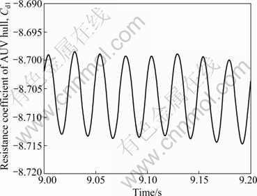
Fig. 8 Change of resistance coefficient of AUV with time

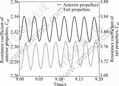
Fig. 9 Changes of resistance coefficient of wheel propellers with time

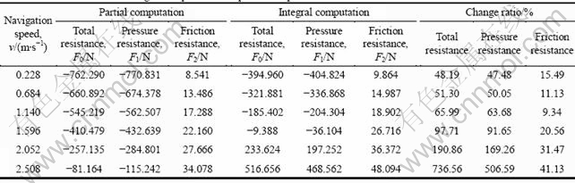
Table 5 gives the resistance of integral computation and partial computation of the viscous flow around the AUV with propellers. As to the unsteady results of integral computation based on sliding mesh, the average resistance of 60 points in three periods is defined as the last resistance result. Due to the mutual interference between the pumping action of wheel propellers and the wake of AUV hull, the total resistance of integral computation increases significantly. The increase of total resistance is mainly from the change of pressure resistance, and friction resistance is almost unchanged. Figures 11 and 12 show that the relative pressure of the AUV with propellers is significantly more than that of AUV without propellers, which reflects the interaction between AUV hull and propellers.

Table 5 Resistance results of integral computation and partial computation

Figures 13 and 14 show the axial velocity distribution of the wake field at x/L=0.876 when the AUV with propellers and the AUV without propellers navigate at 1.14 m/s. Compared with the partial computation, the axial velocity of the wake field of the integral computation increases significantly due to the pumping action and induction of wheel propellers, which indicates that the integral computation can predict the characteristics of the wake field correctly.

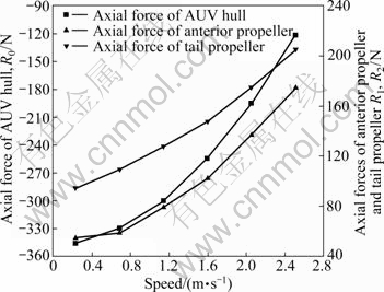
Fig. 10 Axial forces of AUV hull and wheel propellers

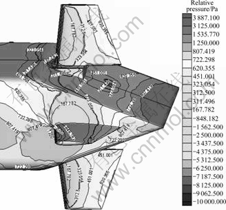
Fig. 11 Relative pressure of AUV with propellers

Figure 15 shows the comparison of relative pressure distribution of pressure side and suction side of wheel propellers between integral computation and partial computation when the wheel propellers navigate at  1.14 m/s. As to the partial computation, the pressure difference between pressure side and suction side is the maximum because there is no interference from AUV hull. While in the case of integral computation, the pressure difference between pressure side and suction side of anterior propellers is significantly less than that of partial computation due to the inflow disturbed by AUV hull. Furthermore, the pressure difference between pressure side and suction side of tail propellers is less than that of anterior propellers under the influence of anterior propellers and AUV hull.

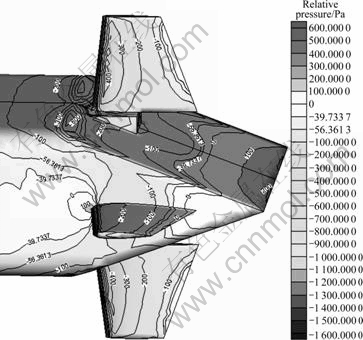
Fig. 12 Relative pressure of AUV without propellers

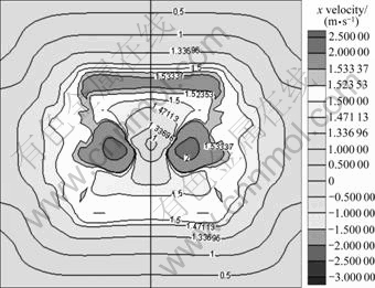
Fig. 13 Axial velocity distribution of wake field of AUV with propellers

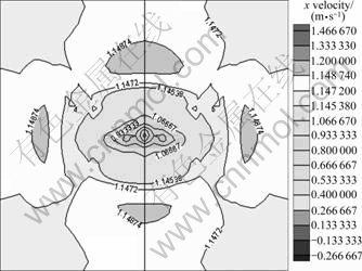
Fig. 14 Axial velocity distribution of wake field of AUV without propellers

Figure 16 shows the computational velocity field at 0.25D behind the propeller plane when the wheel propellers navigate at 1.14 m/s. Compared with the partial computation of wheel propellers, the axial velocity and horizontal velocity of anterior propellers in the integral computation decrease significantly due to the wake of AUV hull. The axial velocity of tail propellers increases compared with anterior propellers, but horizontal velocity decreases, which also shows that the thrust of tail propellers is less than that of anterior propellers.

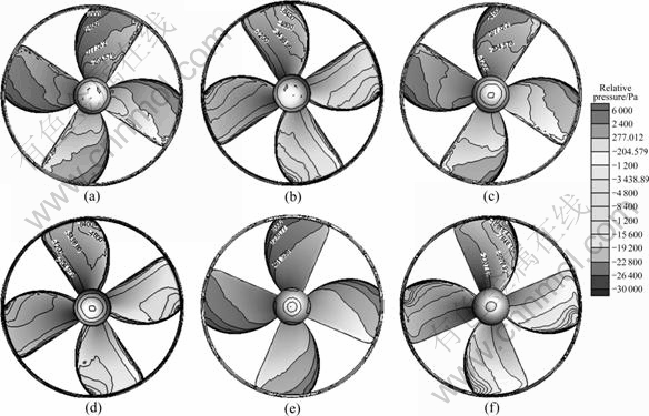
Fig. 15 Relative pressure distribution of pressure side and suction side of wheel propellers: (a) Pressure side of anterior propeller;  (b) Suction side of anterior propeller; (c) Pressure side of tail propeller; (d) Suction side of tail propeller; (e) Pressure side of unattached propeller; (f) Suction side of unattached propeller

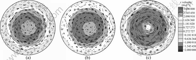
Fig. 16 Computational velocity field at 0.25D behind propeller plane: (a) Anterior propeller; (b) Tail propeller; (c) Unattached propeller

5 Conclusions

1) The CFD method is used to simulate numerically the steady viscous flow around AUV hull and propellers by using the RANS equations, SST k-w model and SIMPLE algorithm based on sub-domains mesh. The computational results agree well with the experimental data, which shows that the numerical method has good accuracy. Base on this, the wheel propeller designed has the characteristics of high thrust, high structural strength, stable hydrodynamic performance and anti-blade flutter, which can meet the design requirements of AUVs’ propellers.

2) Numerical computation is used to simulate the unsteady viscous flow around the AUV with propellers by using RANS equations, SST k-w model and PISO algorithm based on sliding mesh. The results have good convergence. The hydrodynamic characteristics of integral flow field not only reflect the real flow, but also facilitate the study of interaction principle between AUV hull and wheel propellers.

3) The interaction between AUV hull and wheel propellers is predicted qualitatively and quantitatively by comparing the hydrodynamic parameters such as resistance, pressure and velocity with those from integral computation and partial computation of the viscous flow around the AUV with propellers. It provides an effective reference to the study on noise and vibration of AUV hull and propellers in real environment. It also provides technical support for the design of new AUVs.

References

[1] PAN Cun-yun, WEN Xi-sen. Research on Transmission principle and kinematic analysis for involute spherical gear [J]. Chinese Journal of Mechanical Engineering, 2005, 41(5): 1-9.

[2] GAO Fu-dong, PAN Cun-yun, YANG Zheng, FENG Qing-tao. Nonlinear mathematics modeling and analysis of the vectored thruster autonomous underwater vehicle in 6-DOF motions [J]. Journal of Mechanical Engineering, 2011, 47(5): 93-100.

[3] VAN S H, KIM W J. Flow measurement around a model ship with propeller and rudder [J]. Experiments in Fluids, 2006, 40(4): 533-545.

[4] CHOU S K, CHAU S W, CHEN W C. Computations of ship flow around commercial hull forms with free surface or propeller effect [C]// A Workshop on Numerical Ship Hydrodynamics Proceedings. Gothenburg, 2000: 27-35.

[5] PANKAJAKSHAN R, ARABSHAHI A, WHITFIELD D L. Turbofan flow field simulation using Euler equations with body forces [C]// AIAA/SAE/ASME/ASEE 29th Joint Propulsion Conference and Exhibit. Monterey, 1990: 28-30.

[6] XU Jing, GAO Qiu-xin, ZHOU Lian-di. Numerical simulation of Reynolds number effect on effective wake [J]. Journal of Ship Mechanics, 1999, 3(1): 13-20.

[7] ZHANG Zhi-rong, LI Bai-qi, ZHAO Feng. Integral calculation of viscous flow around ship hull with propeller [J]. Journal of Ship Mechanics, 2004, 8(5): 19-26.

[8] Fluent Inc. Fluent user’s guide [M]. Shanghai: Fluent Inc, 2003: 848-857.

[9] SHENG Zhen-bang, YANG Jia-sheng, CAI Yang-ye. Experimental atlas of Chinese ship propellers [M]. Shanghai: Ship Building of China Press, 1983: 28-45.

[10] Hughes M J, KINNAS S A, KERWIN J E. Experimental validation of a ducted propeller analysis method [J]. Journal of Fluids Engineering, 1992, 114(6): 214-219.

[11] GONG Lu, YAO Zheng, WU Man. Numerical analysis for hydraulic characteristics of marine propeller under reverse bent and twist [J]. J. University of Shanghai for Science and Technology, 2007, 29(1): 65-69.

[12] WATANBE T, KAWAMURA T, TAKEKOSHI Y. Simulation of steady and unsteady cavitation on a marine propeller using a RANS CED code [C]// Proceedings of Fifth International Symposium on Cavitation. Osaka, Japan, 2003: 1-4.

[13] FUNEDO I. Analysis of unsteady viscous flow around a highly skewed propeller [J]. Journal of Kansai Society of Naval Architects, 2002, 237: 39-45.

[14] GAO Fu-dong, PAN Cun-yun, CAI Wen-shan, YANG Zheng. Numerical analysis and validation of propeller open-water performance based on CFD [J]. Journal of Mechanical Engineering, 2010, 46(8): 133-139.

[15] GAO Fu-dong, PAN Cun-yun, XU Hai-jun, ZUO Xiao-bo. Design and mechanical performance analysis of a new wheel propeller [J]. Chinese Journal of Mechanical Engineering, 2011, 24(5): 805-812.

(Edited by DENG Lü-xiang)

Foundation item: Project(2006AA09Z235) supported by National High Technology Research and Development Program of China; Project(CX2009B003) supported by Hunan Provincial Innovation Foundation For Postgraduate, China

Received date: 2011-05-28; Accepted date: 2011-09-14

Corresponding author: GAO Fu-dong, PhD Candidate; Tel: +86-731-84574932; E-mail: gaofudong2005@163.com