J. Cent. South Univ. (2017) 24: 988-1001

DOI: 10.1007/s11771-017-3501-1

Parameters studies for rail wear in high-speed railway turnouts by unreplicated saturated factorial design

XU Jing-mang(徐井芒)^{1, 2}, WANG Ping(王平)^{1, 2}, MA Xiao-chuan(马晓川)^{1, 2},

QIAN Yao(钱瑶)^{1, 2}, CHEN Rong(陈嵘)^{1, 2}

1. MOE Key Laboratory of High-speed Railway Engineering, Southwest Jiaotong University, Chengdu 610031, China;

2. School of Civil Engineering, Southwest Jiaotong University, Chengdu 610031, China

Central South University Press and Springer-Verlag Berlin Heidelberg 2017

Abstract: Rail wear is one of the main reasons for reducing the service life of high-speed railway turnouts in China. The rail wear characteristics of high-speed railway turnouts are influenced by a large number of input parameters of the complex train-turnout system. To reproduce the actual operation conditions of railway turnouts, random distributions of these inputs need to be considered in rail wear simulation. For a given nominal layout of the high-speed railway turnout, 19 input parameters for rail wear simulation in high-speed railway turnouts are investigated based on orthogonal design of experiment. Three dynamic responses (wheel-rail friction work, normal contact force and size of contact patch) are defined as observed values and the significant factors (direction of passage, axle load, running speed, friction coefficient, and wheel and rail profiles) are determined by two unreplicated saturated factorial design methods, including the half-normal probability plot method and Dong93 method. As part of the associated rail wear simulation, the influence of the wear models and the local elastic deformation on the rail wear was separately investigated. The calculation results for the wear models are quite different, especially for large creep mode. The local elastic deformation has a large effect on the sliding speed and rail wear and needs to be considered in the rail wear simulation.

Key words: high-speed railway turnouts; rail wear; unreplicated saturated factorial design; wear simulation

1 Introduction

Turnouts are essential components of railway infrastructure, which provide flexibility to traffic operation. They consisted of a switch panel, a movable- point crossing panel and a closure panel for high-speed railway turnouts. To enable the vehicle to change between tracks, the profiles of switch rails and crossing rails are designed to vary along the switch and crossing panels. This leads both to differences in rolling radius and to multipoint contact. The normal wheel-rail contact situations are disturbed when wheels transfer from stock rail to switch rail in the switch panel, or from point rail to wing rail in the crossing panel, sometimes resulting in severe impact loads [1]. Due to the lateral translation of wheelsets and varied rail profiles, dynamic vehicle- turnout interaction is a time variant process; even when discounting track irregularities, it is far more complex than on an ordinary track. These will ultimately lead to serious damage to the contact surfaces and to the transmission of noise and vibrations to the outside environment. In the case of a degraded turnout, severe wear causes major changes in the rail profile, thus having a significant effect on the running behavior of railway vehicles, this may including motion stability, riding comfort and derailment prevention [2, 3]. Railway turnouts contribute to largest part of reported faults and require more maintenance than other parts of the railway network, especially for turnout rail wear. According to statistics from maintenance databases in China [4], it is concluded that one of main reasons for reducing the service life of high-speed railway turnout is severe rail wear. Parts of high-speed railway turnouts changed the switch rails about every one and a half years, much less than design service life (5 years or 150×10⁶ t of total passing weight). Furthermore, failure or disturbance of a turnout may lead to an indirect cost in the form of a traffic shutdown.

The prediction of wheel and rail profile wear is the fundamental issue in railway applications as this can have a direct effect on financing, costs and vehicle safety, especially so for railway turnouts. Much like wheel wear prediction, rail wear prediction methods should also include the dynamic interaction between vehicle and track, as well as an analysis of wheel-rail contact and tribology [5]. Some attempts are made to improve the numerical procedures for wheel and rail predictions on ordinary track. and ZOBORY [6] predicted the profile evolution of wheels and rails considering the material removal to be proportional to the dissipated energy and the specific normal traction distribution, and their simulation also took into account stochastic lateral rail irregularities and stochastic operating conditions. JENDEL [7] developed a wheel profile wear prediction tool based on a load collective concept, in which the actual rail network for the vehicle was reflected by a set of dynamic time-domain simulations and design geometry, and track irregularities, rail profiles and the vehicle operating conditions were considered. performs the simulations of rail wear on four curves with different radii, ranging from 85 to 410 m, but the lubrication of high rail was not considered and the simulated rail wear was more extensive. However, the shapes of the worn rail profile are comparable [8]. ENBLOM and BERG [9, 10] presented a procedure for the simulation of rail and wheel wear, in which the related probabilities of specific vehicle operating conditions and contact parameters and track irregularities were accounted for. The presented procedure is sufficient for an adequate simulation of tread wear, but cannot cover the wear simulation of the flange/gauge corner [9, 10]. BRAGHIN et al [11] presented a fast and reliable wear prediction model to predict railway wheel profile evolution due to wear, in which the vehicle characteristics and a sequence of service conditions were taken into accounted. JIN et al [12] put forward a numerical method to predict curved rail wear during railway vehicle curving, using a combination of Kalker’s non-Hertzian rolling contact theory, the rail material wear model, the coupling dynamics of the vehicle and track, and the three-dimensional contact geometry analysis of wheel-rail. AUCIELLO et al [15] presented a model specially developed for the evaluation of wheel and rail profile evolution. The track is represented by a statistical analysis of the Aosta-Pre Saint Didier line by means of an ensemble of N_c curvilinear tracks, each of length equal to l_track. The statistical analysis has been carried out splitting the considered track in radius classes and superelevation classes. DING et al [14] presented a wheel wear simulation tool to predict wheel wear in heavy haul freight car and the semi-Hertzian method was applied to solve the wheel rail rolling contact. The operations of the car and track were built according to the reliability tests of freight car in China’s Ring-line [14]. WANG and GAO [15] introduced a numerical methodology to simulate the wheel wear evolution of heavy haul freight car. The dynamic simulations were performed separately for all possible track conditions and running velocities in each iterative step to exactly reproduce the actual operating conditions of railway. HAN et al [16] raised a binary numerical wheel wear prediction model of the location on the profile and vehicle operation mileage. The wear coefficients of quartic polynomial were fitted an equation for the location of wear on the profile under a specific operation mileage for the accuracy verification of raised wear prediction model [16]. In the above simulations, several well-developed models were introduced for predicting wheel and rail wear and the operation conditions of vehicle and track were designed to reproduce the actual operating conditions.

The predicted worn profiles are supposed to be uniform along the longitudinal direction of wheel and rail in the wheel-rail wear prediction, and the prediction accuracy is sufficient and accepted for ordinary tangent tracks. However, the varied rail profiles make rail wear variational along the longitudinal direction of railway turnout. The operating reproduction for railway turnout is quite complicated. Dynamic interaction between vehicle and turnout is more complex than on tangent or curved tracks, which leads to the variation of wheel rail contact conditions and rail wear along the turnout’s longitudinal dimension. To obtain a robust simulation results, the input parameters of vehicles and turnouts should be considered variable in the rail wear simulation [17-19]. But the dynamic interaction is affected by a large number of input parameters of vehicles and turnouts. The number of required numerical experiments for factorial design increases with the number of analyzed input parameters by a large margin, and the analysis does not include enough input parameters for the performance of railway turnout. The significant factors are not suitable for rail wear in high-speed railway turnouts. Therefore, two unreplicated saturated factorial design methods, including the half-normal probability plot method and Dong93 method are employed to capture the significant factors, and 19 input parameters for rail wear in high-speed railway turnouts are investigated. As part of the associated rail wear simulation, the influence of local elastic deformation and wear models on the rail wear is separately investigated.

2 Wear simulations

The computation for traditional wheel-rail wear simulation consists of dynamic vehicle-track interaction calculation, wheel-rail rolling contact analysis and material wear model. The dynamic vehicle-track interaction and wheel-rail rolling contact analysis have been developed greatly, and more than 180 types of material wear models have been presented [20]. The main wear models popular in the railway industry include Archard wear model, friction work model and wear index model. In this section, the effects of the wear models and the elastic shear deformation of materials on the calculation of wheel-rail wear are analyzed.

2.1 Wear model

According to studies on different wheel-rail wear tests, many researchers in the world have introduced wheel-rail wear models for wear simulation calculation; however, all wear model principles and test conditions have been different. Therefore, the predicted wheel-rail wear losses are certainly different. An analysis on the difference among the Archard wear model, friction work model and wear index model is shown below. Furthermore, for the sake of contrastive analysis, the wheel-rail normal contact problem is solved with Hertz theory and the tangential contact problem is solved with FASTSIM algorithm.

2.1.1 Archard wear model

Archard wear model was introduced as the sliding friction wear model based on the adhesion wear mechanism thought material wear only occurred in the sliding zone [21]. It is supposed that wear doesn’t occur in the adhesion zone and deducted the following distribution formula corresponding to the wear loss based on many tested results:

                  (1)

where z_sd refers to the wear depth of the contact patch; A refers to the wear area of the contact patch; p_z refers to the contact stress of the contact patch; k_w refers to the wear coefficient, which can be found from the table describing the contact stress and the relative wheel-rail sliding velocity (see Fig. 1). Moreover, △s refers to the relative wheel-rail slippage when the rolling wheel contacts one segment of the contact patch. The calculation formula is as follows:

                       (2)

where △x refers to the length of one segment of the contact patch in the rolling direction and v_r refers to the wheel rolling velocity. In addition, v_x and v_y refer to the longitudinal and transverse relative wheel-rail sliding velocity at one unit of the contact patch.

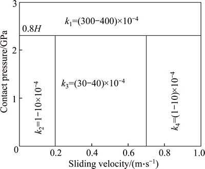
Fig. 1 Wear coefficient of Archard model

2.1.2 Friction work model

Friction work model supposes that wheel-rail wear loss is in relation to the friction work dissipation of the contact patch [22]. It is indicated that not only the sliding zone in the contact patch encounters wheel-rail material wear, but also the adhesion zone has slight wear and peeling. The wheel-rail friction work density for the friction work model is defined as follows:

    (3)

where refers to the friction work density of the contact patch; τ_x(r_p, t) and τ_y(r_p, t) refer to the longitudinal and transverse creepages of the contact patch, respectively; and V_x(r_p, t), V_y(r_p, t) refer to the relative sliding velocity values of the wheel-rail interface of the contact patch, which can be calculated according to the FASTSIM algorithm.

It is indicated that the wheel-rail wear loss can be obtained by multiplying the wear coefficient by the friction work density based on Fig. 2 and following formula:

                         (4)

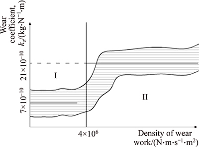
Fig. 2 Wear coefficient of friction work model

2.1.3 Wear index model

Wear index model supposes that the wear loss of the wheel-rail contact patch is in relation to the wear index [11]. The material wear index is defined as follows:

      (5)

where W(x, y) refers to the wear index at the contact patch coordinates (x, y); T_x(x, y) and T_y(x, y) refer to the longitudinal and transverse wheel-rail creep forces at the contact patch coordinates (x, y), respectively; ξ_x(x, y) and ξ_y(x, y) refer to the longitudinal and transverse wheel-rail creepages at the contact patch coordinates (x, y), respectively. Furthermore, A(x, y) refers to the zone area at the contact patch coordinates (x, y). The relation between wear rate and wear index has been obtained based on laboratory tests [11].

2.1.4 Contrast analysis on wear models

In this section, the difference among wheel-rail wear losses of different wear models caused under different creepages is mainly analyzed. The parameters for wear calculation are shown as follows: normal wheel-rail force N=85 kN, friction coefficient f=0.3 and Poisson ratio v=0.25. The radial radii of the wheel and rail are 0.50 m and 0.3 m, respectively. Considering the small creep mode and large creep mode under pure creep and spin creep, the parameter setting with spin creep is as follows. For the small creep mode, the longitudinal creepage ξ₁ and transverse creepage ξ₂ are 0.0012, and the spin creepage ξ₃ is 0.01. For the big creep, the longitudinal creepage ξ₁ and transverse creepage ξ₂ are 0.01, and the spin creepage ξ₃ is 0.5. Under pure creep, the longitudinal creepage ξ₁ and transverse creepage ξ₂ are the same as those tested under spin creep, only changing the spin creepage into 0. The wear loss of the whole contact patch can be obtained by adding the calculated wear loss distribution of the contact patch in the longitudinal axis direction of the contact patch (Figs. 3 and 4).

Fig. 3 Wear distribution in longitudinal direction of contact patch under pure creep:

Fig. 4 Wear distribution in longitudinal direction of contact patch under spin creep:

Regardless of being tested under the small creep mode or large creep mode, the wear loss for the Archard wear model is the highest; for the wear index model, it is lower than the former; and for the friction work wear model, it is the lowest. For pure creep and spin creep, the wear distributions calculated based on the three models are almost the same under the small creep mode, but the wear depth is different, where the wear loss calculated based on the Archard model is 1.23 and 1.39 times those calculated based on the wear index model, respectively, as well as 3.21 and 3.79 times those calculated based on the friction work model, respectively. Under the big creep mode, the wear losses calculated based on the three models are obviously different, where the wear loss calculated based on the Archard model is much higher than that calculated based on the other two wear models (i.e. 7.77 and 7.84 times those calculated based on the wear index model, respectively as well as 19.61 and 19.78 times those calculated based on the friction work model, respectively).

It is clear that different wheel-rail wear models are used based on different test equipments, conditions and environments. Therefore, the results are different to some extent. External conditions (such as normal load, creepage and the friction coefficient) have different effects on different wheel-rail wear models and under the same condition and the calculated results based on the three typical wear models are not the same. In particular, under the large creep mode (full sliding generally), the results always obviously defer from each other for different wear models, where for the Archard model, the result is much higher than that tested based on the other two wear models. Furthermore, the wheel-rail rolling contact problem is solved by the same method in the wear simulation and the input parameters for wear simulation are identical. So, the wear distribution in the simulated results is the same, but the wear depth is quite different. Thus, when the wheel-rail wear is to be estimated and simulated, the selected wheel-rail wear model shall be adjusted according to the measured data in order to ensure the correctness of the simulated result.

2.2 Local elastic deformation on contact surface

The relative wheel-rail sliding velocity at the contact patch interface can be deducted according to the definition of wheel-rail creepage. If only the rigid slippage between wheel and rail is considered, the formula for the relative sliding velocity should be as follows:

                         (6)

If the effect of the elastic shear deformation of wheel-rail materials has to be considered before calculating the relative wheel-rail sliding velocity, the formula for the relative sliding velocity should be as follows.

                    (7)

where u_x and u_y refer to the elastic shear deformation of materials at one point of the wheel-rail contact patch.

In order to analyze the effect of elastic shear deformation of material on the relative motion of the contact interface, the sliding velocity at the contact centre x=0 under pure and spin creep by the small and big creep modes is calculated according to Eqs. (6) and (7). The calculation parameters are shown in Table 1.

For the sliding velocity distribution of contact patches under pure/spin creep (Figs. 5 and 6),

Table 1 Calculation parameters for sliding velocity distribution of contact patch

Fig. 5 Sliding velocity distribution of contact patch under pure creep:

Fig. 6 Sliding velocity distribution of contact patch under spin creep:

Under pure creep, the elastic sliding velocities in the contact patch for both small and large creep modes are higher than the rigid sliding velocity, which can reach up to the highest at the trailing edge of the contact patch and decreases gradually along the longitudinal axis before becoming zero in the adhesion zone. The rigid sliding velocity in the contact patch under pure creep is a constant value before becoming zero suddenly in the adhesion zone. Under spin creep, the elastic sliding velocity in the contact patch is still higher than the rigid sliding velocity. Although its variation law does not change along the longitudinal axis, the rigid sliding velocity in the contact patch is no longer a constant value due to the spin creep and decreases along the longitudinal axis in the sliding zone to some extent. Moreover, it will become zero suddenly in the adhesion zone.

The wear loss distribution of the contact patch can be calculated based on the Archard wear model. Here, the wear loss of the contact patch centre y=0, which is obtained by adding the wear losses of the contact patch along the longitudinal axis direction, is adopted as the overall wear loss distribution of a rail section. To smoothen the contrast analysis, the calculated wear loss results can be processed through normalization. Then, the wear loss distribution of an contact patch under the spin creep can be shown (Fig. 7), and the wear loss distribution of a contact patch under spin creep can be shown (Fig. 8).

Fig. 7 Wear distribution under pure creep:

According to the calculated results, when elastic sliding is considered, the wear losses of the contact patch are higher than those when only rigid siding is considered. Under pure creep, the wear loss of the contact patch is in relation to the symmetric distribution at the x=0 coordinate axis for the contact patch. When elastic sliding is considered, the wear loss of the contact patch will reach up to the peak value at y=0. When only rigid siding is considered, the maximum wear loss of the contact patch will not appear at y=0, but at one position near it. Considering the spin creepage, the wear loss of the contact patch under spin creep is independent of symmetric distribution at the x=0 coordinate axis for the contact patch, and the position with the maximum wear loss is determined by the direction and result of the spin creepage. In addition, for the small creep mode, when elastic sliding is considered, the wear loss of the contact patch will differ greatly from when rigid sliding is considered, namely when elastic sliding is considered, the result will be about 4 times when rigid sliding is considered. For the large creep mode, when elastic sliding is considered, the wear loss of the contact patchwill not change much compared with the case that when rigid sliding is considered. In other words, when elastic sliding is considered, the wear loss of the contact patch will be 1.36 times when rigid sliding is considered. Under large creep mode, the rigid slippage of the contact patch is almost the same as the elastic slippage and the rigid sliding plays a major role. Meanwhile, under the small creep mode, the rigid slippage of the contact patch differs greatly from the elastic slippage. Therefore, the effect of elastic shear deformation must be considered when the wheel-rail wear is calculated under the small creep mode; otherwise, the result will be relatively low.

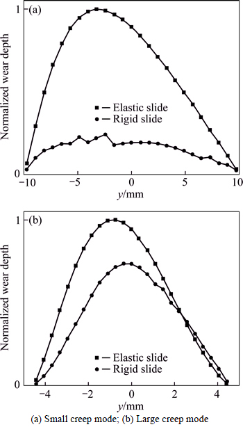
Fig. 8 Wear distribution under spin creep:

3 Parameter studies

The wear characteristics of turnout rails are mainly dependent on the dynamic interaction between vehicle and turnout, while the latter is affected by the parameters with regard to the vehicle system, turnout track system and wheel-rail contact. However, the effects of different system parameters on turnout rail wear are not quite clear. In this work, according to the main effect analysis methods adopted widely in fields such as biological pharmacy and electronic information, key dynamic parameters with regard to turnout rail wear are screened according to the orthogonal table based Plackett-Burman saturated unreplicated factorial design method [23] in order to perform a predictive simulation of the turnout rail wear and an optimized design of the turnout structure. The vehicle-turnout dynamic interaction is simulated using the validated commercial software Simpack. The simulated vehicle model is based on a three-dimensional multi-body model of the Chinese CRH2 high-speed vehicle and the simulated turnout model is based on a standard CN60-1100-1:18 turnout design for high-speed railway.

3.1 Unreplicated saturated factorial design method

3.1.1 Effect model

For saturated factorial design, a linear model is always used as its effect model. The linear effect model is expressed as follows [24]:

                                 (8)

where Y=(y₁, y₂, …, y_m)^T refers to the observed value array; β=(β₀, β₁, …, β_m-1)^T refers to the unknown parameter to be calculated; β₀ refers to the mean of observed values. Moreover, β₁, β₂, …, β_m-1 refers to the effect of analysis factors; X refers to the matrix of m×m, X=(I_m, X_m-1)^T; I_m refers to the unit column vector of m dimension, and X_m-1=(x₁, x₂, …, x_m-1) is determined by the unreplicated saturated test design. Furthermore, x_i (i=1, …, m-1) refers to the array of m dimension; ε=(ε₁, ε₂, …, ε_m)^T refers to the error array of the test, and m refers to the designed frequency for the test. The statistical model for saturated factorial design should also meet the following hypotheses:

① The test error array data of ε_i (i=1, 2, …, m) are independent random variables and have the same mean value and mean-square deviation, where the mean value and mean-square deviation are 0 and σ, respectively;

② All test error array data of ε_i (i=1, 2, …, m) meet the normal distribution, namely ε~N (0, σ²);

③ For β_i (i=1, 2, …, m-1), at most, t(1≤t≤m) is zero. In other words, at most, t analysis factors whose effects are not zero are within m-1.

For the orthogonal test design, if Hypothesis ① is satisfied, the optimized variance linear unbiased estimation of the analysis factor effect β can be obtained easily as follows:

                           (9)

If the test design satisfies Hypothesis ②, the optimized variance linear unbiased estimation will also be appropriate for the normal distribution and the mathematical expectation and mean-square deviation of

which are β_i and respectively and the (i=1, 2, …, m-1) values are independent from each other.

The factorial design aims to study and analyze whether the analysis factors have an active effect, that is, if any active member can be found within the contrasts through a specified analysis method based on m observed value arrays, namely Y=(y₁, y₂, …, y_m)^T.

                    (10)

                           (11)

To test Eq. (9), if H₀ is not tenable, then analysis factors with an active effect can be found, which can be identified through factor selection [23].

3.1.2 Graphical analysis method

Graphical analysis methods are adopted to analyze active effect factors through a graphic solution, where the half-normal (or normal) probability graph method presented by DANIEL in 1959 [25] and improved by ZAHN [26] is popular in selecting factors. As the estimated effect values of analysis factors are dispersed in probability distribution graphs, error might arise when selecting the significant factors. However, the estimated factor effect values in half-normal probability plot are set as absolute; therefore, the above errors can be prevented, and the active effect factors can be selected with ease.

The half-normal probability plot method is established based on half-normal distribution. Supposing a random variable is X, the random variable X satisfies the half-normal distribution, namely X~HN(τ²). When τ²=1, the random variable X satisfies the standard half-normal distribution, which can be expressed as X~HN(1). If the statistical model for the saturated factorial design can satisfy Eq. (10) and H₀ is tenable, the optimized variance linear unbiased estimation of the analysis factor effect will satisfy the normal distribution, namely

Half-normal probability plot method is used for selecting significant factors through discrimination lines. Firstly, the factor effect value (i=1, 2, …, m) is estimated based on the observed values. After being selected, the absolute values can be sorted in an ascending order, and thus, the statistic sort of can be obtained. Then, the quantile q_j of the standard half-normal distribution HN(1) can be calculated. The point pair j=1, 2, …, m distribution of the half-normal probability plot can be drawn by taking the factor effect values as the x-axis and the corresponding quantiles as the y-axis. Finally, the significant factors can be identified by using the discrimination line. If some points are not on the discrimination line obviously, the corresponding factors can be considered as significant.

3.1.3 Dong93 method

The half-normal probability plot method can be adopted to discriminate significant factors visually; however, to a certain extent, experience is still important. For example, the distance between an effect point pair and a straight line for identifying significant factors is not normalized. Therefore, in a sense, half-normal probability plot method can only be adopted for discriminating the existence of significant factors rather than identifying them exactly. The numerical analysis method is characterized by objective discrimination and reliable conclusions and adopted as a complement of the half-normal probability plot method in order to further identify significant factors. In this work, the Dong93 method is adopted for determining significant factors.

DONG [27] indicated that amended standard error (e_ASE) can be adopted for estimating the effect mean- square deviation σ shown as

             (12)

where m_inactive refers to the number of effect factors of The active effect of the estimated factor effect value can be determined according to

                          (13)

where If the estimated effect value of one factor meets the above formula, this factor can be considered as significant; otherwise, it is insignificant.

3.2 Orthogonal design of experiment

The elements affecting the dynamic performance of the vehicle-turnout system are selected as analysis factors in the study in order to determine the effect of different elements on the vehicle-turnout system and select those main effect factors that can obviously affect the turnout rail wear behaviour. In this work, 19 factors (such as the direction of train passing through turnout zone, speed of train passing through turnout zone, nominal wheel radius and rail gauge at turnout zone) are adopted in the analysis (see Table 2).

In Table 2, the affecting element F₁ refers to the direction of the train passing through the turnout zone. In addition, different levels of the affecting element F₂-F₆ and F₁₃-F₁₉ have specific parameters; therefore, F₁-F₆ and F₁₃-F₁₉ can be inputted conveniently in the dynamic model of the vehicle-turnout system. Moreover, different levels of the affecting element F₇-F₁₂ are hard to be expressed with parameters and therefore are defined in this work.

The wheel profile and turnout rail profile are shown with different levels (Fig. 9), where the nominal wheel and turnout rail profile are obtained from the designed drawings. The wheel and turnout rail profile with wear losses are measured with a Miniprof wheel-rail profile measuring instrument.

Table 2 Analysis on factor levels of elements affecting turnout rail wear

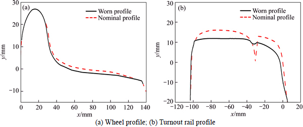
Fig. 9 Definitions for wheel profile and turnout rail profile with different levels:

Affecting elements F₉-F₁₂ are adopted to study the effect of the geometric irregularity of turnout zones on the turnout rail wear. Generally, the geometric irregularity distribution of rails, to a certain extent, is stochastic; therefore, its features should be described via the power spectrum density function. However, the power spectrum density function can only be adopted to describe the statistical wavelength and amplitude laws and features with regard to rail irregularity. Thus, when the dynamic analysis on the wheel-rail system is performed, the power spectrum density function should be transformed into the corresponding time domain specimen for the rail irregularity through a Fourier transform in order to adopt it as an excitory input. In this work, the level-5 track spectrum (USA) is adopted to simulate the random geometric irregularity (Fig. 10).

After the level of effect factors with regard to turnout rail wear is analyzed, the most import evaluation indexes affecting the turnout rail wear behaviour can be determined. According to the analysis on the wheel-rail wear calculation model, the most important indexes affecting turnout rail wear behaviour are considered the following three items: wheel-rail friction work (expressed as W=F_xξ_x+F_yξ_y, namely the product of contact patch creep force and corresponding creepage), normal wheel-rail contact force (expressed as T, namely the summation of forces being perpendicular to the contact patch plane) and wheel-rail contact patch area (expressed as A=A_a+A_s consisting of the sliding zone and adhesion zone). Taking the Archard wear model as example, the formula involves the normal wheel-rail contact force, the wheel-rail contact patch area and the relative sliding velocity of the wheel-rail particle on the contact patch interface and so on, where the normal wheel-rail contact force and contact patch area can be adopted to determine the material wear directly. The relative sliding velocity of the wheel-rail particle on the contact patch interface can be reflected by the wheel-rail friction work indirectly; therefore, in this work, the above three dynamic responses are adopted as the observed vectors of the statistical model to select significant effect factors.

Fig. 10 Stochastic irregularity definition:

For the selected 19 analysis factors affecting the turnout wear behaviour, the L₂₀(2¹⁹)-based saturated unreplicated factorial design method is adopted in order to test them 20 times (see Table 3 for a detailed test plan, “+” stands for high level, “-” stands for low level). A simulation calculation for the test is conducted based on the dynamic model for vehicle-turnout system, according to previous work [28]. After the calculated dynamic response results with regard to the observed values of wheel-rail friction work, normal wheel-rail contact force and wheel-rail contact patch area and so on are adopted as the designed test values for the statistical analysis model and the designed test values are processed based on the corresponding graph methods or numerical analysis method. Furthermore, the 19 analysis factors can be selected in order to obtain the significant effect factors. The dynamic response results with regard to the observed values are also shown (see Table 4).

3.3 Significant factors screening

The dynamic response results can be adopted as the observed values for the factorial design. Since the orthogonal design based saturated unreplicated factorial design method is adopted in this work and only two levels with regard to each factor are analyzed, the optimized variance linear unbiased estimation for all factor effects will also be appropriate for the normal distribution. Its mathematical expectation and mean-square deviation are β_i andrespectively. The effect estimation of all parameters can be calculated according to Eq. (8) in order to select active effect factors. The effect estimation of different parameters is also shown (Table 5). In Table 5, “error” stands for the error effect estimate of effect factor, due to the specific algorithm of unreplicated saturated factorial design method [23].

Table 3 Unreplicated saturated test design plan for turnout rail wear behaviour

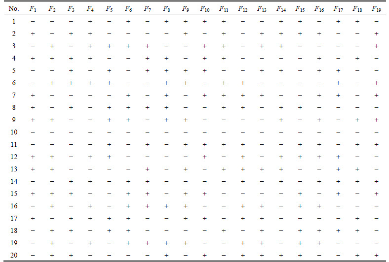
Table 4 Calculated dynamic response results of observed values

3.3.1 Half-normal probability plot method

By taking the calculated results (Table 5) as the x-axis of half-normal probability plot, the half-normal probability values of factors can be calculated according to Eq. (9). In addition, the half-normal probability distribution graphs of wheel-rail friction work, normal force and wheel-rail contact patch can be obtained (Fig. 11), where the blocks refer to the estimated absolute values of different effect factors and the triangles refer to an incorrect estimation of the effect factors.

For half-normal probability plots, significant factors are screened according to the discrimination line. If one point is far from the discrimination line as compared with most of the points, then it can be considered an active effect factor. Significant factors of wheel-rail friction work, normal force and wheel-rail contact patch can be screened as listed in Table 6.

Table 5 Effect estimation of different parameters

3.3.2 Dong93 method

The Dong93 method was adopted for further screening of significant factors in order to ensure the correctness selection according to half-normal probability plots. For this method, the amended standard error (ASE) was adopted to estimate the effect mean- square deviation σ (see Table 7 for the detailed results). It is an analysis method with low probability for zero error, and therefore, during the selection, some significant factors might be ignored, causing less active effect factors as compared with the actual number and even significant factors without any response values.

3.3.3 Significant factors

Since the Dong93 method can only be adopted to select those factors with an obvious effect, the significant factors of wheel-rail contact patch cannot be screened. This method can only be considered a complement for the results selected based upon half-normal probability plots. Therefore, in this work, the results selected based upon half-normal probability plots are dominant. According to the half-normal probability distribution graphs and Dong (1993) method, key factors affecting the turnout rail wear behaviour are the direction of trainpassing through turnout zone, the speed of vehicle passing through turnout zone, the vehicle axle load, the wheel-rail friction coefficient and wheel and rail profiles.

Fig. 11 Half-normal probability plots:

Table 6 Significant factors for dynamic response

Table 7 Screening of significant factors based on Dong93 method

4 Conclusions

1) Existing numerical prediction methods for wheel and rail profiles evolution are reviewed. To reproduce the actual operating conditions in the simulation, the simulation of vehicle-track dynamic interaction was particularly performed. For high-speed railway turnouts, dynamic interaction between vehicle and turnout is more complex than tangent or curved tracks, leading to variations in wheel-rail contact and rail wear along the turnout’s longitudinal dimension. The rails wear characteristics are influenced by a large number of input parameters of the complex train-turnout system.

2) Both the wear models and the local elastic deformation have a large effect on rail wear simulations. Different wear models are deduced based on different test equipments, conditions and environments. It shall be corrected based on the field measurement for ease of rail wear simulations in high-speed railway turnouts in China. The local elastic deformation at the wheel-rail interface affects the sliding speed and rail wear remarkably and needs to be considered in the rail wear simulation.

3) For a given nominal layout of the high-speed railway turnout, 19 input parameters for rail wear in high-speed railway turnouts are investigated based on orthogonal design of experiment. Three dynamic responses (wheel-rail friction work, normal contact force and size of contact patch) are defined as observed values. Two unreplicated saturated factorial design methods, including the half-normal probability plot method and Dong93 method, are used to screen the significant factors. It has been shown that direction of passage, axle load, running speed, friction coefficient, and wheel and rail profiles have the largest effects on the rail wear in high-speed railway turnouts.

4) The significant factors are considered to be stochastic for performing the actual operation conditions of railway turnouts in the rail wear simulation. The outcome of this article could provide theoretical guidance for optimization of the turnout design and modify dynamic performance of the vehicle and thus increase ride quality.

References

[1] XU Jing-mang, WANG Ping, MA Xiao-chuan, XIAO Jie-ling, CHEN Rong. Comparison of calculation methods for wheel-switch rail normal and tangential contact [J]. Proceedings of the Institution of Mechanical Engineers, Part F: Journal of Rail and Rapid Transit, 2016, (DOI: 10.1177/ 0954409715624939)

[2] LAGOS R F, ALONSO A, VINOLAS J. Development of a real-time wheel-rail contact model in NUCARS and application to diamond crossing and turnout design simulations [J]. Proceedings of the Institution of Mechanical Engineers, Part F: Journal of Rail and Rapid Transit, 2012, 226(6): 587-602.

[3] SUN Y Q, COLE C, MCCLANACHAN M. The calculation of wheel impact force due to the interaction between vehicle and a turnout [J]. Proceedings of the Institution of Mechanical Engineers, Part F: Journal of Rail and Rapid Transit, 2010, 224(5): 391-403.

[4] XU Jing-mang, WANG Ping. The investigation report on the damage of railway turnouts-field survey and measurement [R]. Chengdu: School of Civil Engineering, Southwest Jiaotong University, 2014. (in Chinese)

[5] TUNNA J, SINCLAIR J, PEREZ J. A review of wheel wear and rolling contact fatigue [J]. Proceedings of the Institution of Mechanical Engineers, Part F: Journal of Rail and Rapid Transit, 2007, 221(2): 271-289.

[6] A, ZOBORY I. On deterministic and stochastic simulation of wheel and rail profile wear process [J]. Periodica Polytechnica: Transportation Engineering, 1998, 26(1, 2): 3-17.

[7] JENDEL T. Prediction of wheel profile wear-comparisons with field measurements [J]. Wear, 2002, 253(1, 2): 89-99.

[8] A. Simulation of rail wear on the Swedish light rail line [D]. Stockholm: Department of Aeronautical and Vehicle Engineering, Royal Institute of Technology (KTH), 2005.

[9] ENBLOM R, BERG M. Simulation of railway wheel profile development due to wear-influence of disc braking and contact environment [J]. Wear, 2005, 258(1, 2): 1055-1063.

[10] ENBLOM R, BERG M. Proposed procedure and trial simulation of rail profile evolution due to uniform wear [J]. Proceedings of the Institution of Mechanical Engineers, Part F: Journal of Rail and Rapid Transit, 2008, 222(1): 15-25.

[11] BRAGHIN F, LEWIS R, DWYER R S. A mathematical model to predict railway wheel profile evolution due to wear [J]. Wear, 2006, 261(11, 12): 1253-1264.

[12] JIN Xue-song, WEN Ze-feng, XIAO Xin-biao, ZHOU Zhong-rong. A numerical method for prediction of curved rail wear [J]. Multibody System Dynamics, 2007, 18(4): 531-557.

[13] AUCIELLO J, IGNESTI M, MALVEZZI M, MELI E, RINDI A. Development and validation of a wear model for the analysis of the wheel profile evolution in railway vehicles [J]. Vehicle System Dynamics, 2012, 50(11): 1707-1734.

[14] DING Jun-jun, LI Fu, HUANG Yun-hua, SUN Shu-lei, ZHANG Li-xia. Application of the semi-Hertzian method to the prediction of wheel wear in heavy haul freight car [J]. Wear, 2014, 314(1, 2): 104-110.

[15] WANG Pu, GAO Liang. Numerical simulation of wheel wear evolution for heavy haul railway [J]. Journal of Central South University, 2015, 22(1): 196-207.

[16] HAN Peng, ZHANG Wei-hua, LI Yan. Wear characteristics and prediction of wheel profiles in high-speed trains [J]. Journal of Central South University, 2015, 22(8): 3232-3238.

[17] JOHANSSON A, PALSSON A B, EKH M, NIELSEN J C, ANDER M K, BROUZOULIS J, KASSA E. Simulation of wheel-rail contact and damage in switches &crossings [J]. Wear, 2011, 271(1, 2): 472-481.

[18] NICHLISCH D, KASSA E, NIELSEN J, EKH M, IWNICKI S. Geometry and stiffness optimization for switches and crossings, and simulation of material degradation [J]. Proceedings of the Institution of Mechanical Engineers, Part F: Journal of Rail and Rapid Transit, 2010, 224(4): 279-292.

[19] KASSA E, NIELSEN J C O. Stochastic analysis of dynamic interaction between train and railway turnout [J]. Vehicle System Dynamics, 2008, 46 (5): 429-449.

[20] ENBLOM R. Deterioration mechanisms in the wheel–rail interface with focus on wear prediction: A literature review [J]. Vehicle System Dynamics, 2009, 47 (6): 661-700.

[21] ARCHARD J F. Contact and rubbing of flat surfaces [J]. Journal of Applied Physics, 1953, 24(8): 981-988.

[22] ZOBORY I. Prediction of wheel/rail profile wear [J]. Vehicle System Dynamics, 1997, 28(2): 221-259.

[23] HOU Shu-juan, DONG Duo, REN Li-li, HAN Xu. Multivariable crashworthiness optimization of vehicle body by unreplicated saturated factorial design [J]. Structural and Multidisciplinary Optimization, 2012, 46(6): 891-905.

[24] CHEN Ying, KUNERT J. A new quantitative method for analyzing unreplicated factorial designs [J]. Biometrical Journal, 2004, 46(1): 125-140.

[25] DANIEL C. Use of Half-normal plots in interpreting factorial two-level experiments [J]. Technometrics, 1959, 4(1): 311-341.

[26] ZAHN D A. An empirical study of the half-normal plot [J]. Technometrics, 1975, 17(2): 201-211.

[27] DONG F. On the identification of active contrasts in unreplicated fractional factorials [J]. Statist. Sinica, 1993, 37(l): 209-217.

[28] XU Jing-mang, WANG Ping, WANG Li, CHENG Rong. Effects of profile wear on wheel-rail contact conditions and dynamic interaction of vehicle and turnout [J]. Advances in Mechanical Engineering, 2016, 8(1): 1-14.

(Edited by YANG Hua)

Cite this article as: XU Jing-mang, WANG Ping, MA Xiao-chuan, QIAN Yao, CHEN Rong. Parameters studies for rail wear in high-speed railway turnouts by unreplicated saturated factorial design [J]. Journal of Central South University, 2017, 24(4): 988-1001. DOI: 10.1007/s11771-017-3501-1.

Foundation item: Projects(51425804, 51378439, 51608459) supported by the National Natural Science Foundation of China; Projects(U1334203, U1234201) supported by the Key Project of the China’s High-Speed Railway United Fund; Project(2016M590898) supported by China Postdoctoral Science Foundation; Project(2014GZ0009) supported by Sichuan Provinial Science and Technology support Program, China

Received date: 2016-03-30; Accepted date: 2017-01-10

Corresponding author: CHEN Rong, Associate Professor; Tel: +86-13699008192; E-mail: chenrong@home.swjtu.edu.cn