J. Cent. South Univ. (2017) 24: 1344-1350
DOI: 10.1007/s11771-017-3538-1

Short-term travel flow prediction method based on FCM-clustering and ELM
WANG Xing-chao(НхРЗі¬)1, HU Jian-ming(єъјбГч)2, LIANG Wei(БєО°)2, ZHANG Yi(ХЕТг)2
1. Department of Control Science and Engineering, Tongji University, Shanghai 201804, China;
2. Department of Automation, Tsinghua University, Beijing 100084, China
 Central South University Press and Springer-Verlag Berlin Heidelberg 2017
Abstract: Short-term travel flow prediction has been the core of the intelligent transport systems (ITS). An advanced method based on fuzzy C-means (FCM) and extreme learning machine (ELM) has been discussed by analyzing prediction model. First, this model takes advantages of ability to adapt to nonlinear systems and the fast speed of ELM algorithm. Second, with FCM-clustering function, this novel model can get the clusters and the membership in the same cluster, which means that the associated observation points have been chosen. Therefore, the spatial relations can be used by giving the weight to every observation points when the model trains and tests the ELM. Third, by analyzing the actual data in Haining City in 2016, the feasibility and advantages of FCM-ELM prediction model have been shown when compared with other prediction algorithms.
Key words: intelligent transportation systems (ITS); travel flow prediction; extreme learning machine (ELM); FCM-clustering; spatio-temporal relation
1 Introduction
With the rapid development of the economy, the number of vehicles has increased and traffic jam has been the prominent problem which arouses the world-wide concern. In recent decades, the management and control in transportation system, especially the intelligent transportation system (ITS), has been merged as the key solution for soothing the severely worsening traffic congestion. In small-medium cities the transportation jam problem is more serious than before. Road short term travel prediction takes an important role in the ITS to ease the pressure of transportation. Traditional short term travel prediction models include: Kalman filter [1], auto-regressive integrated moving average model (ARIMA), neural networks, support vector regression (SVR). Besides, the neural networks method has been another major tool to predict the travel flow.
Nevertheless, these current prediction models have the obvious fault. When the research studies the time series model, the researchers always assume that the time is linear, but the actual trend is nonlinear, which leads to lack of reliability of these models. Besides, some artificial intelligent models, like neural networks, can fit nonlinear systems. However, the neural networks have some obvious shortcomings like over fitting, complex network structure and iteration training to find the rational weight [2]. Compared with these traditional forecasting models, ELM has smaller weights norm and faster speed to forecast [3]. Since 2006, a variety of studies have been developed in many fields. In fields as data classification [4] and classification [5], they are all based on application of ELM. LI and CHEN [6] proposed a model of WNN-ELM for 1-month ahead discharge forecasting. ELM algorithm is also applied in multivariate chaotic time series prediction [7]. Thus, ELM algorithm can perform better when it is used to forecast the short-term travel flow.
Moreover, the current majority of research on travel-flow prediction is based on time series theory. Therefore, these predicting models do not cover the spatial information. Although many prediction models based on time series have already been developed [8], the travel flow is not only related to the time series but also related to the adjacent roads. Therefore, if we only consider the time series and ignore some spatial information among adjacent roads, the prediction models may be not perfect.
Furthermore, before using the ELM to forecast the travel flow, the clustering function is used to divide the observation points into several clusters. These observation points which are in the same cluster have similar properties. Thus, when the research combines theses data in case of the relationship between different points, the training set of the ELM will be more reliable than other time-series models. Compared with other clustering function, FCM-Clustering function is the better complete function. FCM-Clustering bases on the objective function [9]. It does not only divide data into different clusters, it also offers the membership between data and the clustering center. We can give rational weight to different observation points in case of these memberships when we combine the training data.
For further accuracy, rapidity and stability of travel flow prediction, the FCM-ELM model has been used to predict the travel flow in this paper. This research covers the relationship between different observation points. Therefore, the prediction algorithm does not only cover the space-time relations but also takes advantage of the ELM modelЎЇs fast speed and ability to adapt to the nonlinear systems.
2 FCM-clustering and ELM
2.1 FCM-clustering
The fuzzy C-means (FCM) method was performed by the Bezdek, which allows data to belong to an improvement of two or more clusters [9].
Theorem 1:X={x1, x2, Ў, xn} is a dataset, which can be divided. FCM algorithm divides xi into different clusters(c) whose centers can get the minimum value of the objective function. The minimum of the following function is the foundation of this algorithm:
 (1)
(1)
where uijЎК(0, 1), the center of the cluster can be displaced as ci. And the distance between the ith clustering center and the jth data point can be indicated as dij=||ci-xj||. mЎК[1, ЎЮ) means pointsЎЇ weight. The sum of the membership is equal to 1, which is the configuration factor
 (2)
(2)
Derived from the Lagrangian multiplier method, we can build the following functions:

 (3)
(3)
Over all, the essential conditions to attain the minimum in Eq. (1) are:
 (4)
(4)
 (5)
(5)
Steps of FCM algorithm are
1) Initialize the matrix U;
2) Calculate the centers by Eq. (4);
3) Renew U(k), U(k+1) by Eq. (5);
4) Judge the condition  stop.
stop.
2.2 Extreme learning machine algorithm
The ELM algorithm is a fast learning method [3]. This method is a kind of single-layer feedforward neural networks (SLFNs). The reason why the weight of input can be randomly settled is that the activation function in the hidden layer can be infinitely differentiated. Moreover, the least squares solutions can be obtained by minimizing quadratic loss function [10]. As a result, the iteration is not needed when the network parameters are under randomly determining, which benefits the reducing of the amount of calculation and the time of forecasting. The network structure of ELM shows in Fig. 1 [11].
Theorem 2: For N different samples, which can be displayed as (xi, ti), xi=[xi1, xi2,  , xin]T means the input vector belongs to Rn(n is the number of input node). And ti=[ti1, ti2,., tim]T means the output vector belongs to Rm. The activation function can be displayed as G(x). The following function can display the property of the model for j=1, 2, Ў, N.
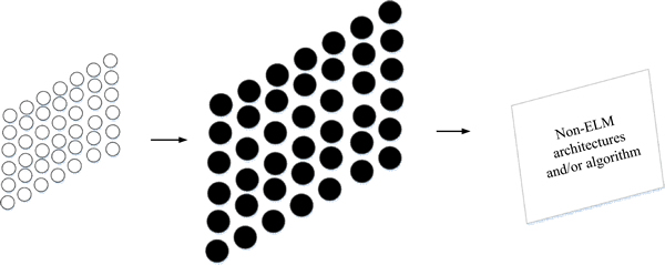
Fig. 1 ELM algorithm diagram
 (6)
(6)
where the value vector connected the ith hidden node and the input layer nodes can be presented as ¦Шi=[¦Шi1, ¦Шi2, Ў, ¦Шin]T. And bi is the threshold of the ith hidden layer node. ¦Вi=[¦Вi1, ¦Вi2, Ў, ¦Вim]T is the weight vector, which connects the hidden layer and the output layer. When simplifying these N connecting equations, the model can be attained as following equation.
 (7)
(7)
 (8)
(8)
 (9)
(9)
 (10)
(10)
where H means value matrix of the hidden layer output and ¦В is the output layer weight vector. T means the desired output matrix and k is the output node number. H+ can be attained by the Moore-Penrose generalized inverse. The H is the MP inverseЎЇs original matrix. Thus, the least squares solution of Eq. (7) can be calculated as
 (11)
(11)
Steps of ELM algorithm:
1) Random assignment of input weights and hidden layer thresholds;
2) With MP algorithm, attain the value of the hidden layer output vector H;
3) By Eq. (11), attain the value of the output weights vector ¦В.
3 Prediction algorithm based on FCM and ELM
In this prediction algorithm, FCM is the tool to cluster different observation points into several clusters. The input of clustering is the data of 13 observation points. With FCM-clustering, we can obtain the relationship among all observation points.
When we want to forecast the (j+1)th sequence data, we can get the jth traffic flow data. It is that there are N daysЎЇ data and one day has T sequences. Therefore, the data vector is NЎ¤T and the ith observation pointЎЇs jth traffic flow data is xij.
By using the FCM function, these I observation points will be clustered into n clusters. Moreover, this function will give the membership matrix U, which means the relations between the observation point and the center. Thus, we can set the weight vn of every point in the same cluster by the matrix U to combine the data matrix. This calculation will update the input matrix.
The new xij should be
 (12)
(12)
where xiЎЇjЎЇ is the observation pointsЎЇ data in the same cluster and vn is the weight of xiЎЇjЎЇ. What we want to attain is xN,j+1.
The training input of ELM is:
 (13)
(13)
The training output is:
 (14)
(14)
The testing input is:
 (15)
(15)
The whole structure of FCM-ELM algorithm is shown in Fig. 2.
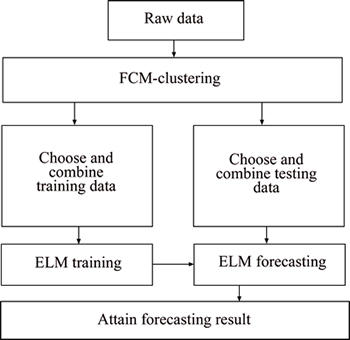
Fig. 2 Steps of FCM-ELM algorithm
4 Data analysis and results
4.1 Experimental dataset
In this work, the raw data is gathered in Haining County, Jiaxing City, Zhejiang Province, China, by microwave in 2016. The continue flow data have been detected all days and the detection interval is 1 min. These test data cover 20 d and one day has 1440 sequences. Moreover, 13 observation points have been selected in the test. These observation pointsЎЇ locations are shown in Fig. 3.
In this case, the first 19 days data are training data and the 20th day data are testing data. Nevertheless, when the experiment compares the raw travel-flow data in Haining City with the large citiesЎЇ, following pictures can show the different properties:
Small-medial cities have several different properties compared with the large cities: fewer travel-flow volumes; Stronger fluctuation; No obvious crest.
If only the raw data are used to forecast, this experiment cannot get accurate conclusion for these properties. For example, if the real travel-flow value is 0 and the forecasting value is 1, the calculating accuracy will be influenced. Therefore, the research cuts out the data from 500th point to 1000th point and these points will be used in the experiment. Besides, strong fluctuation will influence the forecasting process. Thus, the experiment uses the merge function to merge 5 points into 1 point so that the detection interval is 5 min. The merged data show as following picture:
The forecasting process is programmed in Matlab 2014a environment running in an Intel Core i5-3230M, 2.6 GHz CPU. Running the program with the history data and testing data will get the forecasting performance.
4.2 Clustering result
The research analyzes the data from 8 a.m. to 5 p.m.(the data from 500th point to 1000th point) by FCM- Clustering, because more valid information contained in these data. Thus, the experiment can attain the clustering results shown in Table 1.
By using the FCM function, the research can get the membership between observation points. Thus, the weight of every observation point has been determined.
4.3 Prediction results and analysis
This section will give the results which are attained by the Matlab 2014a. These results are shown in Table 3 and Fig. 6. Auto-regressive integrated moving average model (ARIMA) is a traditional time series prediction model which has shown the good performance in prediction. Simple ELM just use the raw data to train and test the ELM. And wavelet neural network (WNN) is the usual network to predict. BP (back propagation) neural network is a multi-layer feedforward neural network trained by error back propagation algorithm, which is the most widely used neural network. These three models will be the comparisons with the FCM-ELM to find whether this model can predict better.
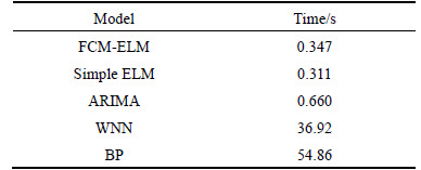
4.3.1 Calculating time
Firstly, this experiment compares this model with simple ELM, wavelet neural network (WNN) and auto-regressive integrated moving average model (ARIMA) in the speed aspect. In this test, the 4th observation point is chosen to forecast separately. The result shows in Table 2.
From the comparison in Table 2 between FCM-ELM model and other models, the conclusion can be obvious offered that the forecasting speed of this model is faster. Although the simple ELM is faster 0.03 s than this model, but the FCM-ELM has to calculate the combining process. WhatЎЇs more, time is a part of evaluation parameters, the accuracy will be tested in the following section. Moreover, WNNЎЇs process time included training time is so long that it must occupy too much time to calculate. Thus, the FCM-ELM modelЎЇs speed can be proved fast.

Fig. 3 Distribution of observation points
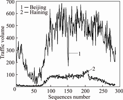
Fig. 3 Traffic-flow data in Haining and Beijing

Fig. 5 Merged data
Table 1 Clusters
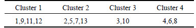
Table 2 Processing time comparison
Secondly, this research also tests the ability to calculate the prediction of other 12 observation points to know whether this model can apply to the actual environment. Because the real transport system is great and the model should have the ability to calculate many observation points at the same time. Therefore, other 12 observation points are tested at the same time and the results show in the following picture. And this process just cost 1.213 s which is short enough.
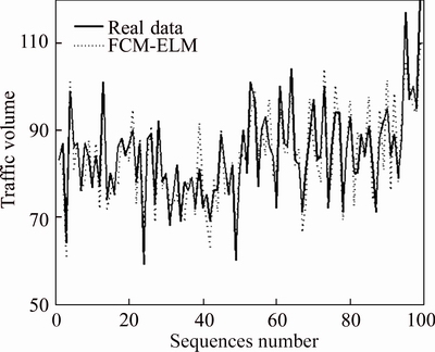
Fig. 6 FCM-ELM forecasting result
4.3.2 Forecasting accuracy
In this section, this research also chooses the 4th observation point to be the forecasting point. Compared with simple ELM, WNN, BP and ARIMA, the accuracy can be tested, and the accuracy of every model is shown in Fig. 8 and Table 3.
From this comparison with ELM, WNN and ARIMA, the conclusion can be easily discussed that the accuracy of FCM-ELM prediction algorithm is better than othersЎЇ. The time-space relation helps the ELM to use the data with spatial information. And the abilities of ELM help the algorithm to adapt to this nonlinear system. Therefore, the performance of ELM is good for predicting based on uniform sampling data.
We also consider the different methods to cover the relations between observation points. This method, called direct ELM, does not give the weight of every observation points but all data belonged to a same cluster will be the input of ELM to train and test this network. However, the result showed in Fig. 9 cannot satisfy the need of actual application because the accuracy is lower than othersЎЇ. The error rate is 14.80%. The reason caused this situation is the relationship may be not tight. And overmuch data low the prediction accuracy. Therefore, setting the weight according to the membership which is calculated by FCM will help the ELM to get better prediction accuracy.
6 Conclusions
1) With FCM clustering, the raw data have been clustered to several clusters whose relationships are close.
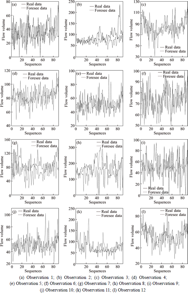
Fig. 7 Other 12 observation forecasting results:
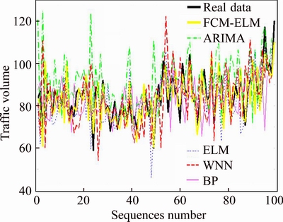
Fig. 8 Comparison of forecasting methods
Table 4 comparison in accuracy
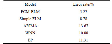
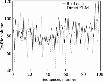
Fig. 9 Direct FCM-ELM prediction result
In case of the membership which is calculated from the FCM clustering function, the process will determine the weight, which means the relationship among the observation points clustered in the same cluster.
2) The new data are formed by summarizing all observation pointsЎЇ data. By using ELM prediction method, we can predict the short term traffic volume data faster and more accurate.
3) By analyzing the actual data in Haining city in 2016, the advantages of FCM-ELM prediction model have been shown by comparing with other algorithms. This character can remedy the shortcoming which other models exist. Notably, this model can provide better support for traffic guidance in the ITS.
References
[1] ZHU T, KONG X, LV W. Large-scale travel time prediction for urban arterial roads based on kalman filter [C]// 2009 International Conference on Computational Intelligence and Software Engineering, Wuhan, China: ICCISE, 2009:1-5. doi: 10.1109/CISE.2009.5365441
[2] LI L, WANG D, XIAO Z, LI X. Urban road travel time prediction based on ELM [C]// International Conference on Advanced Materials and Computer Science. Qingdao, China: ICAMCS, 2016: 392-395. doi:10.2991/icamcs-16.2016.83
[3] HUGAN G B, ZHU Q Y, SIEW C K. Extreme learning machine: Theory and applications [J]. Neurocomputing, 2006, 70(1-3): 489-501.
[4] DING X J, CHANG B F. Active set strategy of optimized extreme learning machine [J]. Science Bulletin, 2014, 59(31): 4152-4160.
[5] FENG L, WANG J, LIU S, XIAO Y. Multi-label dimensionality reduction and classification with extreme learning machines [J]. Journal of Systems Engineering and Electronics, 2014, 25(3): 502-513.
[6] LI B J, CHENG C T. Monthly discharge forecasting using wavelet neural networks with extreme learning machine [J]. Science China Technological Sciences, 2014, 57(12): 2441-2452.
[7] HAN M, ZHANG R, XU M. Multivariate chaotic time series prediction based on ELMЁCPLSR and hybrid variable selection algorithm [J]. Neural Processing Letters, 2017: 1-13.
[8] PAN F, ZHAO H B. Online sequential extreme learning machine based multilayer perception with output self feedback for time series prediction [J]. Journal of Shanghai Jiaotong University (Science), 2013, 18(3): 366-375.
[9] BEZDEK J C, EHRLICH R, FULL W. FCM: The fuzzy C-means clustering algorithm [J]. Computers & Geosciences, 1984, 10(2, 3): 191-203.
[10] HUANG G B. What are extreme learning machines? filling the gap between frank rosenblattЎЇs dream and john von neumannЎЇs puzzle [J]. Cognitive Computation, 2015, 7(3): 263-278.
[11] DENG C W, HUNAG G B, XU J, TANG JX. Extreme learning machines: new trends and applications [J]. Science China Information Sciences, 2015, 58(2): 1-16.
[12] XU Long-qin, Combined prediction model of water temperature in industrialized cultivation based on empirical mode decomposition and extreme learning machine [J]. Journal of Agricultural Mechanization, 2016, 47(4): 265-271.
(Edited by DENG LЁ№-xiang)
Cite this article as: WANG Xing-chao, HU Jian-ming, LIANG Wei, ZHANG Yi. Short-term travel flow prediction method based on FCM-Clustering and ELM [J]. Journal of Central South University, 2017, 24(6): 1344-1350. DOI: 10.1007/s11771-017-3538-1.
Foundation item: Project(2016YFB0100906) supported by the National Key R & D Program in China; Project(2014BAG03B01) supported by the National Science and Technology Support plan Project China; Project(61673232) supported by the National Natural Science Foundation of China; Projects(DlS11090028000, D171100006417003) supported by Beijing Municipal Science and Technology Program, China
Received date: 2016-12-15; Accepted date: 2017-04-01
Corresponding author: HU Jian-ming, PhD, Associate Professor; Tel: +86-10-62794001; E-mail: hujm@mail.tsinghua.edu.cn

