J. Cent. South Univ. (2016) 23: 850-858

DOI: 10.1007/s11771-016-3132-y

Relay movement control for maintaining connectivity in aeronautical ad hoc networks

LI Jie(李杰)^{1, 2}, SUN Zhi-qiang(孙志强)¹, SHI Bo-hao(师博浩)³, GONG Er-ling(宫二玲)¹, XIE Hong-wei(谢红卫)¹

1. College of Mechatronic Engineering and Automation, National University of Defense Technology,

Changsha 410073, China;

2. Beijing Aeronautical Technology Research Center, Beijing 100076, China;

3. School of Business, Central South University, Changsha 410083, China

 Central South University Press and Springer-Verlag Berlin Heidelberg 2016

Abstract: As a new sort of mobile ad hoc network (MANET), aeronautical ad hoc network (AANET) has fleet-moving airborne nodes (ANs) and suffers from frequent network partitioning due to the rapid-changing topology. In this work, the additional relay nodes (RNs) is employed to repair the network and maintain connectivity in AANET. As ANs move, RNs need to move as well in order to re-establish the topology as quickly as possible. The network model and problem definition are firstly given, and then an online approach for RNs’ movement control is presented to make ANs achieve certain connectivity requirement during run time. By defining the minimum cost feasible moving matrix (MCFM), a fast algorithm is proposed for RNs’ movement control problem. Simulations demonstrate that the proposed algorithm outperforms other control approaches in the highly-dynamic environment and is of great potential to be applied in AANET.

Key words: aeronautical ad hoc network (AANET); mobile ad hoc networks; topology control; network connectivity; movement control

1 Introduction

As a new research field, aeronautical ad hoc network (AANET) [1] is mainly comprised of aircraft in the airspace, and satellites or ground stations can also be considered important parts of the AANET. The ground station may be a control center or relay station, and the satellite may be used for long distance or emergency data communication. Due to the self-organizing multi-hop feature, AANET can greatly expand the connectivity over the line-of-sight (LOS) limitation of radio wave and the limitation of transmission range. In civil aviation, data communications through AANET can provide the internet connection and periodic downloads of black box data in real time [2-4]. In military fields, current military airborne networks provide only their own mission specific implementations, and provide limited interoperability and autonomous routing capability. AANET technology is expected to satisfy the stringent requirements of military airborne networks, such as high network dynamics, bandwidth efficiency, security, and robustness [5].

In AANET, airborne nodes (ANs) are moving at a very high speed and the network is highly dynamic with constantly changing topology. Due to the high speed and limited communication range of ANs, AANET may suffer from frequent network partitioning. Moreover, in a harsh environment, the damage to AANET can also partition the network into disjoint segments. For example in a battle field, ANs in hostile conditions are susceptible to fail, after which the surviving nodes may be grouped into disjoint partitioned networks. Therefore, the end-to- end connectivity in AANET cannot be guaranteed, and the communication will be disrupted frequently. The delay-tolerant/disruption-tolerant network (DTN) architecture [6] can be used to provide reliable data transmission in challenged networks similar to AANET that suffer from high delay, frequent interruption and limited node resources. The most distinguish feature of DTN is its store-carry-forward routing paradigm. By this paradigm, messages will be carried by routing nodes instead of discarding if there is no available network connection in a short period. However, most applications of AANET are delay-sensitive (e.g., VoIP, tactical information exchanging, and other security-related applications), and DTN architecture cannot guarantee a low delay for these real time services.

As an important technique to maintain a certain level connectivity for networks, topology control can be used to guarantee the end-to-end connectivity in AANET. The connectivity level of a network can be described in graph theory by means of vertex connectivity. A graph is said to be k-vertex connected if for every pair of nodes, there are at least k vertex-disjoint paths connecting them. A network is said to be simply connected if the connectivity level k=1, and to be fault tolerant if k≥2. Topology control can be mainly implemented in three ways. The first way is adjusting the nodes’ transmission power to conserve energy meanwhile maintain network connectivity, and this way is mainly used in wireless sensor network (WSN) [7-8]. Due to ANs’ limited transmission power and sparse distribution in a wider area, AANET may not achieve a specified connectivity even if all ANs use the maximum transmission power. Hence, the first way of topology control cannot be applicable for AANET. If all the nodes are controllable, the second way of topology control can be used via controlling the nodes’ movement to re-establish the topology [9]. However, the second way is also not suitable for AANET, because ANs move depending on the objective that they try to achieve and we cannot control the ANs’ movement. The third way of topology control is to add one or more relay nodes in the network to restore the network connectivity [10-11]. In this wrok, we use the third way to control the network topology. To improve the connectivity of AANET, additional relay nodes (RNs) (e.g., unmanned aerial vehicles (UAVs) and high-altitude airships) are needed [12]. Also, since ANs are mobile, it is necessary to re-configure the communication topology by RNs’ movement. As ANs move, RNs need to move as well and it is desirable to move them a minimum amount to re-establish the topology as quickly as possible, e.g., we should determine the instantaneous speeds of all RNs during the run time to maintain the network a specified level of connectivity with a minimum total movement of existing RNs. OUYANG et al [13] proposed an optimal design for UAV path planning to guarantee the connectivity in the scenario where a UAV is used as relay between a mobile access point and a fixed base station. However, the proposed method [13] cannot guarantee a certain level connectivity for a network formed by multiple mobile terminal nodes.

There have been some recent works in restoring connectivity for the network by the movement of relay nodes [14-15]. KASHYAP and SHAYMAN [14] proposed algorithms for minimizing the number of additional nodes required and the distance that they need to move for construction of a topology with desired levels of connectivity. The algorithm forms a complete graph on the terminal nodes and weights the edges of the graph according to a weight function. Then, it computes an approximately minimum weight spanning k-vertex connected subgraph of the complete graph. Finally, the maximum weight matching is used to move the exiting relay nodes to the new relay positions such that the total movement is minimized. Since the results of relay nodes’ movement are figured out based on the current network topology, network topology may change to a new state when the relay nodes arrived at the new relay position in the highly-dynamic environment. Thus, the algorithm proposed [14] is not suitable for the highly-dynamic aeronautical environment. SENTURK et al [15] proposed a distributed force-based approach to guarantee network recovery for partitioned networks by minimizing the movement cost of the relay nodes [15]. Force-based approach is based on the idea of magnetic repelling force in physics. All the relay nodes are assumed to be polarized with the same magnetic pole and push each other to move. Force-based approach works well for re-connecting the partitions; however, it cannot realize a specified k-vertex connected network.

This work proposes an online algorithm for RNs’ movement control to maintain AANET k-vertex connected in the highly-dynamic aeronautical environment. The network model and problem definition are firstly given, and then, the online movement control algorithm is presented by defining the minimum cost feasible moving matrix (MCFM). A fast algorithm for seeking MCFM is thus proposed. Simulation and result analysis are discussed finally.

2 Network model and problem statement

For simplicity, we assume that all the aircraft cruise at the same cruising altitude, and then the problem can be studied in a two-dimensional space. It is assumed that there are w ANs and m RNs on the two-dimensional Euclidean plane. RNs are identical to the ANs in terms of their transmission range and type of links. Let r be the communication range of ANs and RNs. The set of ANs is denoted by V_A={a₁, a₂, …, a_w}, where a_i, (1≤i≤w), represents the i-th AN. The set of RNs is denoted by V_R= {r₁, r₂, …, r_m}, where r_j, (1≤j≤m), represents the j-th RN. In this work, a letter in bold denotes the position vector of the node represented by the same letter, i.e., the position of AN a_i is represented by the vector a_i=(x_ai, y_ai) and that of RN r_j is represented by the vector r_j=(x_rj, y_rj), where x_ai, y_ai, x_rj and y_rj are the absolute node coordinates. Matrix A=[a₁, a₂, …, a_w] represents the positions of ANs in V_A, and matrix R=[r₁, r₂, …, r_m] represents that of RNs in V_R. The velocity vector of RN r_i at time t is denoted by v_i(t), and then the velocities of RNs in V_R at time t can be denoted by matrix V(t)=[v₁(t), v₂(t), …, v_m(t)]. The objective of the problem is to figure out the velocity matrix V(t), 0A is at least k-vertex connected in the resulting graph G=(V_A∪V_R, E), where E is the set of links between the nodes that are within each other’s transmission range. This problem can be formulated as the following optimized model.

                       (1)

            (2)

    (3)

where ||v_i(t)|| denotes the magnitude of velocity vector v_i(t); λ_t(u, v) is the number of vertex-disjoint paths between u and v in G at time t; and v_max is the maximum velocity of RNs. In most cases, AANET is uncertain, i.e., ANs’ future state is unknown. Then, the whole problem data from the beginning is unavailable, and we cannot find exact solutions of the constrained optimization Eqs. (1)-(3) in an offline fashion. Therefore, an online approach for RN’s movement control is needed. Figure 1 shows the framework of the online movement control approach. Let A(t) and R(t) represent positions of ANs and RNs at time t, respectively. Instantaneous speeds of ANs at time t are denoted by . The network’s state at time t can be determined by A(t),  and R(t). Based on the network’s actual state and the desired connectivity level k, the controller calculates RNs’ velocities V(t) at time t such that the set of ANs V_A can keep k-vertex connected and RNs can travel a short total distance during the run-time T.

3 Online movement control algorithm

In this section, we describe an online optimization approach for RNs’ movement control. Firstly, we process Eqs. (1)-(3) with the discrete manner which can be rewritten as follows:

               (4)

   (5)

 (6)

where △t is the sample interval, V[n]=[v₁[n], v₂[n], …,v_m[n]], n=0, 1, ..., K, is the sampling data of V(t);  denotes the maximum value of n; and λ_n(u, v) is sampling data of λ_t(u, v). Obviously, the result of mode (4) will be reasonably small if v_i[n] is determined such that the value of is the minimum for n=0,1, ..., K. Thus, we can find an online method to determine v_i[n] as follows: According to velocities and positions of ANs at time n, the positions of ANs at time n+1 can be estimated. Then, based on the positions of RNs at time n and the estimated positions of ANs at timen+1, v_i[n] can be determined such that is the minimum, meanwhile the set of ANs V_A is at least k-vertex connected in the network constructed by ANs with the estimated positions and RNs with the new positions after moving.

Definition 1: Let RN r_i move according to a moving vector d_i, and RNs in V_R move according to a moving matrix D=[d₁, d₂, …, d_m]. For the 5-tuple (k, V_A, A, V_R, R), the feasible moving matrix is a moving matrix D if the set of ANs is at least k-vertex connected in the network constructed by ANs with position A and RNs with the new position R+D after moving. A feasible moving matrix D is called a minimum cost feasible moving matrix (MCFM) for (k, V_A, A, V_R, R) if the valueof is the minimum among all feasible moving matrixes for (k, V_A, A, V_R, R). The problem to seek a MCFM for (k, V_A, A, V_R, R) is called MCFM(k, V_A, A, V_R, R) problem or MCFM problem for short.

Let A[n]=[a₁[n], a₂[n], …, a_w[n]] and R[n]=[r₁[n], r₂[n], …, r_m[n]] be the positions of ANs and RNs at time n respectively. Let be the instantaneous speeds of ANs at time n. If network’s accurate state can be obtained in real time, i.e., A[n], and R[n] can be obtained accurately at time n, our online approach for RNs’ movement control can be described by Algorithm 1. Aircraft is commonly equipped with satellite communication terminals for emergency communication. Then, the state information of each aircraft can be delivered to the control center via satellite communications. Algorithm 1 is mainly divided into two parts. In the first part, velocities of ANs are assumed to remain constant during time △t, and new positions of ANs after time △t are estimated. In the second part, as the core of the algorithm, MCFM problem is solved. To our knowledge, the MCFM problem is NP-hard and has never been studied before. Since the movement control algorithm is running online, there is much need for a “real time” algorithm for MCFM problem. Thus, a method that is simpler, faster, and able to run online should be found to solve MCFM problem.

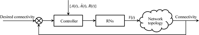
Fig. 1 Online movement control

Algorithm 1: Online approach for RNs’ movement control

1) Get the value of A[n], and R[n] at time n.

2) Estimate the positions of ANs at time n +1, as below:.

3) Call MCFM(k, V_A, V_R, R[n]) to compute the minimum cost feasible moving matrix of RNs at time n (denoted by D[n]).

4) Set V[n] = D[n]/△t. If V[n] has a velocity v_i[n] whose magnitude is higher than v_max, set ||v_i[n]|| = v_max.

5) n ← n +1.

6) Goto 1.

4 Fast algorithm for MCFM problem

The algorithm for MCFM problem is based on a concept known as steinerization, which was first introduced by LIN and XUE [16] and widely used in relay node placement problems [17]. For two nodes x and y on the plane with the positions x and y respectively, if ||x-y||≤r, x and y can communicate with each other directly; If ||x-y||>r, we can connect x and y by deploying a minimum number of relays on the line segment [x, y] (steinerizing [x, y]) and we call these relays’ positions as steiner points (SPs). If ||x-y||>r, we steinerize [x, y] by setting SPs on the line segment [x, y] and these SPs evenly divide the segment [x, y] intosegments. The set of SPs steinerizing [x, y] is denoted by V_S[x, y]. Obviously, if ||x-y||≤r,  V_S[x, y]=. Given a communication range r and a set of nodes V, the set of SPs for the 2-tuple (V, r), denoted by S(V, r), is given by

                 (7)

For the set V_A, we assume that S(V_A, r)={s₁, s₂, …, s_h}, where s_i represents the ith SP. S(V_A, r) can be regarded as the set of candidate locations for RNs to move. The position of SP s_i is represented by the vector s_i=(x_si, y_si), where x_si and y_si are the absolute node coordinates. Then, MCFM(k, V_A, A, V_R, R) problem can be considered an optimal assignment problem that SPs in S(V_A, r) are assigned to RNs in V_R so that the RNs can move a minimum total distance to the assigned SPs and the set of ANs V_A is at least k-vertex connected after RNs’ moving.

Figure 2 illustrates a network with 4 ANs and 3 RNs, i.e., V_A={a₁, a₂, a₃, a₄} and V_R={r₁, r₂, r₃}. Since the distance between a₄ and any other ANs is longer than the transmission range r, all ANs construct a disconnected network. We study the problem MCFM(k, V_A, A, V_R, R) with k=1. To restore the connectivity, RNs in V_R can move to some SPs in set S(V_A, r)={s₁, s₂, s₃, s₄, s₅, s₆, s₇} and make the network at least simple connected. As shown in Fig. 2, when r₁ moves to the position of s₁, r₂ moves to the position of s₂ and r₃ stays still, the RNs can move a minimum total distance, meanwhile the network’s connectivity is guaranteed. Then, moving matrix D=[s₁-r₁, s₂-r₂, 0] can be regarded as the MCFM, i.e., MCFM(1, V_A, A, V_R, R)=[s₁-r₁, s₂-r₂, 0].

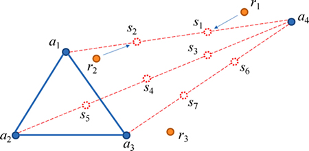
Fig. 2 MCFM problem

In a square region with length L, the total number of SPs |S(V_A, r)| = O(L|V_A|²/r). Suppose that |V_R| ≤ |S(V_A, r)|, the total number of assignments is larger than |S(V_A, r)|!/(|S(V_A, r)| - |V_R|)!. Thus, when L, |V_R| and |V_A| are large, it is hardly to obtain the best answer by using common enumeration in a limited time. The proposed algorithm [14] constructs a weighted complete graph on the terminal nodes whose edges are weighted according to edges’ length, and then finds the potential relay locations by computing an approximately minimum weight spanning k-vertex connected subgraph of the complete graph. However, this method can only find the minimum number of potential relay locations needed to form a k-vertex connected subgraph, and cannot guarantee that the relay nodes move to those potential relay locations with the minimum total distance. In the combinatorial optimization problem, it is hard to find a weight function for edges that can accurately represent the cost of RNs’ movement. Furthermore, the guaranteed α-approximation algorithms for k-connected subgraphs [18] are based upon solving linear programs, and are difficult to implement in the online fashion which requires the implementations to be simpler and faster. Therefore, approaches via finding the minimum cost spanning subgraph do not suit our online RNs’ movement control algorithm. In this work, we use the concept of matching in the graph theory to solve the MCFM problem.

A matching in a graph is a set of non-loop edges with no shared endpoints, and a maximum matching is a matching of maximum size among all matchings in the graph [19]. Considering the complete bipartite graph  with vertex set V(K)=V_R∪S(V_A, r) and edge set E(K), a matching M in  can determine a moving matrix D=[d₁, d₂, …, d_m] for RNs in V_R. For a moving vector d_i in the moving matrix D, if the RN r_i∈ V_R is matched to a SP s_j∈S(V_A, r) in the matching M, the vector d_i is set to be s_j-r_i; otherwise, 0. Take the network illustrated in Fig. 2 for example, the complete bipartite graph  with partite sets V_R and S(V_A, r) is shown in Fig. 3. For , the edge set with no shared endpoints (e.g., {r₁s₁, r₂s₂},{r₂s₃, r₃s₇}and{r₁s₄, r₂s₃, r₃s₇}) is defined as a matching in , and the minimum cost feasible moving matrix D=[s₁-r₁, s₂-r₂, 0] is determined by the matching M={r₁s₁, r₂s₂}. We weight each edge in  according to the distance from the corresponding RNs to SPs. For an edge r_is_j ∈ E(K), the weight function W(r_is_j) is defined as

         (8)

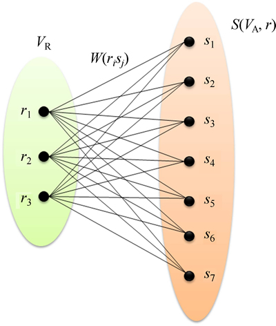
Fig. 3 Complete bipartite graph

For the weighted bipartite graph , the maximum weighted matching is a maximum matching with the maximum total weight. The Kuhn-Munkres algorithm [19] provides a polynomial-time approach for calculating the maximum weighted matching. Therefore, we can repeatedly perform maximum weighted matching on  to find the potential relay locations where RNs can move to with a short total distance and make the set of ANs at least k-vertex connected.

The fast approach for MCFM problem shown as Algorithm 2 mainly consists of three phases. In the first phase (Steps 1-10), the Kuhn-Munkres algorithm is used to perform maximum weighted matching on the weighted bipartite graph  to get a matching M*. The set of SPs in S(V_A, r) that are matched by M* is denoted by Matched(S(V_A, r), M*). The SPs in Matched(S(V_A, r), M*) are added to the original graph G=(V_A, E(G)). These SPs are allowed to form edges with all vertices of G in range r and the resulting graph is tested for k-vertex connectivity. If the resulting graph is not k-vertex connectivity, the algorithm sets S(V_A, r)= S(V_A, r)-Matched(S(V_A, r), M*), and continually adds SPs from S(V_A, r) to the resulting graph by the aforementioned method until the resulting graph is at least k-vertex connected. Let V_C denote the set of SPs that have been added to the original graph G. Obviously, RNs can move to them with a relatively short total distance to construct a k-vertex connected network. However, some SPs in V_C are redundant for the k-vertex connected network, and should be removed from V_C.

Algorithm 2: Fast algorithm for MCFM(k, V_A, A, V_R, R)

Input: k, V_A, A, V_R, R

Output: D=[d₁, d₂, …, d_m]

1:  Set V_C ←, V_S ←S(V_A, r).

2:  while (1) do

3:  Construct a complete edge weighted bipartite graph

4:  Perform maximum weight matching on  to get a mach M*.

5:  V_C ←V_C∪Matched(V_S, M*)

6:  if G=(V_A ∪ V_C, E(G)) is at least k-vertex connected then

7:  break

8:  end if

9:   V_S ←V_S - Matched(V_S, M*)

10:  end while

11:  for s ∈ V_C in decreasing order of c(s) do

12:  if G’=(V_A∪V_C-{s}, E(G’)) is at least k-vertex connected then

13:  V_C←V_C-{s}

14:  end if

15:  end for

16:  Construct a complete edge weighted bipartite graph K_{|VR|, |VC|}.

17:  Perform minimum weight matching on K_{|VR|, |VC|} to get a matching M.

18:  for each r_i ∈V_R do

19:  if r_i is matched to s ∈ V_C by M then

20:  set d =s-r_i

21:  else

22:  set d_i=0

23:  end if

24:  end for

In the second phase (steps 11-15), redundant SPs are removed from V_C to minimize the number of potential relay locations. For a SP s_i∈V_C, the cost of s_i, denoted by c(s_i), is defined as the average distance from current positions of RNs to s_i, i.e.

                   (9)

The algorithm repeatedly attempts to remove SPs from V_C, in decreasing order by weight c(s), but putting the SPs back if it is necessary for k-vertex connectivity. Experimentally, this pruning stage can remove 60%-80% of the added SPs. The resulting subgraph G’= (V_A∪V_C, E(G’)) is therefore at least k-vertex connected and RNs can easily realize it with a short total distance.

In the last phase (steps 16-24), the weighted bipartite graph with vertex set V_R∪V_C is constructed. Each edge in  is weighted according to Eq. (8), and then, the algorithm performs maximum weighted matching on  to get a matching M which can determine a moving matrix D with relatively low cost for (k, V_A, A, V_R, R).

Steps 1-15 in Algorithm 2 are similar to the greedy solution for k-vertex connected subgraph proposed in Ref. [20]. Unlike the greedy solution repeatedly adding edges to the graph in increasing order by the weight of edges, Algorithm 2 adds the SPs to the original graph by performing maximum weight matching repeatedly, and the SPs added to the graph early have lower cost than those added later. After Step 15, Algorithm 2 finds relative small amount of SPs that can make the network k-vertex connected, and meanwhile, RNs can move a low total distance to them. However, the algorithm can have arbitrary poor performance. Figure 4 depicts a disconnected network has two RNs (r₁ and r₂) and three ANs (a₁, a₂ and a₃). All ANs are equidistance from each other and the distance between any two ANs is 1.5r. The centre of the equilateral triangle formed by the three ANs is denoted by s, and its position vector is denoted by s. To repair the connectivity (k=1), the moving matrix calculated by Algorithm 2 is [s₁-r₁, s₂-r₂], i.e., r₁ moves to the position of s₁ and r₂ moves to the position of s₂. However, the optimal solution is [s-r₁, 0], i.e., r₁ moves to the position of s and r₂ stays still. Since the value (||s₁-r₁||+||s₂-r₂||)/||s-r₁|| can be arbitrarily large, the ratio of the worst-case cost to optimal is unbounded.

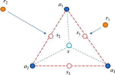
Fig. 4 Example of poor performance by Algorithm 2

The total number of edges in G=(V_A, E(G)) is O(|V_A|²) and the maximum number of SPs on any edge in E(G) is O(L/r) in a square region with length L, thus, the total number of SPs |V_S|=O(L|V_A|²/r). The maximum weighted matching on a bipartite graph of n vertices takes O(n^2.5) time and connectivity test for a undirected graph with m nodes takes O(m²) times, thus, steps 3-9 in Algorithm 2 take O(|V_S|^2.5) time. In the worst case, steps 3-9 may repeat |V_S|/|V_R| times, so steps 2-10 take O(|V_S|^3.5/|V_R|) times. Steps 11-15 takes O(|V_S|³) times and steps 16-24 take O(|V_S|^2.5 + |V_r|) times. Therefore, the total times required for Algorithm 2 are O(|V_S|^3.5/|V_R|+ |V_R|)=O(L^3.5|V_A|⁷/(r^3.5|V_R|)+|V_R|).

5 Performance evaluation

5.1 Simulation setup

We assume that there are w ANs moving at a speed v in a square region with a side of length 400 km to perform a special task. Each AN has a relatively short transmission range of 90 km. In order to improve the connectivity, m RNs with a maximum speed of 600 m/s are added to the network. RNs have the same transmission range and link type as ANs. The network model is implemented on OMNeT++ simulation platform [21]. In order to represent the movement patterns of the aircraft more accurately, each AN follows random-waypoint mobility model [22] and the pause times are set to zero. The total simulation time is set to be 40 min. Since k≥3 is usually considered not worth the additional cost, only the cases for simple connected (k=1) and fault-tolerant (k=2) are studied in the simulation. Generally, AANET is a sparse network which has a relative small number of ANs in a limited region, so the large scalar network is not considered in the simulation. Since it is difficult for a aircraft to achieve sustained supersonic cruise in the current technology level,     we assume that all ANs fly at a subsonic speed.   Figure 5 shows a snapshot of the network topology,where w=12, m=2, k=1 and v=250 m/s.

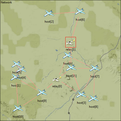
Fig. 5 Snapshot of network topology

The following metrics are used to measure the performance of the proposed approach.

1) Total travel distance (TTD): TTD (D_TT) indicates the total distance traveled by all the RNs during the running time. Movement demands high energy consumption and impacts the overall network lifetime. Therefore, it is important to reduce the travel distance.

2) Connectivity rate (R_C): R_C indicates the proportion of the time when the network’s connectivity is higher than a specific level to the total simulation time. The proportion of the time when the network is at least k-vertex connected to the total simulation time is denoted by R_C-k. The objective of movement control algorithm is to guarantee the network a specific level of connectivity, and can directly show the control effects.

3) Relative connectivity rate (RCR): When m RNs are added to the network with w ANs to maintain the network k-vertex connected, the increase in R_C-k is partly due to the increase of node density. Thus, another performance metric, RCR, is defined to avoid the effect of node density on the network connectivity. For a certain value of k, R_CR-k of a network with w ANs and m RNs can be computed as: R_CR-k=R_C-k-R_C-k(w+m), where R_C-k(w+m) denotes the value of R_C-k in a network only with w+m ANs.

△t is an important parameter which greatly affects the performance and should be determined first. In Algorithm 1, we assume that the velocities of ANs are kept constant in △t, but this assumption will be invalid if △t is too large. Moreover, a too large △t also decreases the control times T/△t during the run time T. Considering that the maximum distance a RN can move in △t is v_max△t, if △t is too small, some RNs cannot reach their destinations after △t, which may influence the control effects. Therefore, we should find a proper value for △t according to dynamics of the network. We set w=12, m= 5, k=2, and varied △t when the ANs moving at different speed v. Figure 6 shows R_C-2 (Fig. 6(a)) and TTD (Fig. 6(b)) as a function of △t when the network is low (v=100 m/s) and high (v=300 m/s) dynamic. We can see that the best performance can be achieved at about △t= 15 s for the low dynamic network and at about △t=20 s for the high dynamic network. In the experiments, we set △t=17 s.

5.2 Experiment results

5.2.1 Performance analysis

We set v=200 m/s, w=12, and varied the number of RNs to analyze performance of the control algorithm. Figure 7 shows the values of R_C-1 and R_C-2 as a function of RNs’ number when the control algorithm guarantees the network simple connected (k=1) and fault-tolerant (k=2) respectively. As shown in Fig. 7, for k=1, R_C-1 increases obviously with the number of RNs increasing whereas R_C-2 is not significantly enhanced; and for k=2, R_C-2 increases obviously than R_C-1 with the number of RNs increasing. Thus, the proposed algorithm can significantly enhance the connectivity rate for the desired connectivity level.

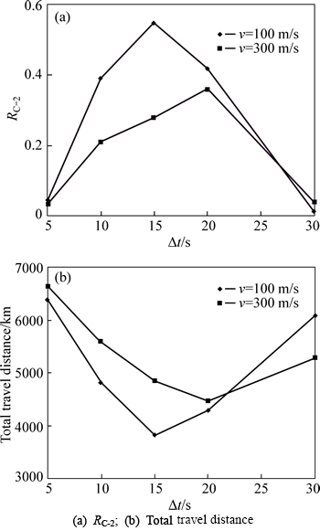
Fig. 6 Performances as a function of △t:

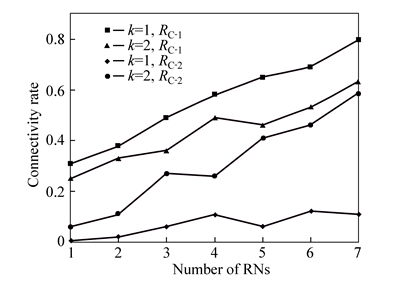
Fig. 7 Connectivity rate as a function of RNs’ number

When RNs are added to the network, the increase in connectivity rate of the network is partly due to the increase of node density. In order to avoid the effect of node density on the network connectivity, we then study another performance metric, R_CR, which can directly indicate the increase in connectivity rate only due to the control algorithm. Figure 8 shows the values of R_CR-1 and R_CR-2 as a function of RNs’ number when the control algorithm guarantees the network simple connected and fault-tolerant respectively. We can notice that R_CR-1 and R_CR-2 do not increase monotonically with increasing RNs’ number, and they have a peak when RNs’ number is set to be 3 and 5 respectively. This means that the control algorithm works best for simple connectivity when 3 RNs are added, and for fault-tolerance when 5 RNs are added.

Figure 9 shows the value of D_TT as a function of RNs’ number for k=1 and 2 respectively. As shown in  Fig. 9, the D_TT does not increase obviously with the number of RNs increasing when RNs is more than 3 for k=1 and 5 for k=2. This is because if there are enough RNs added to the network, node density will be high enough to maintain the desired network’s connectivity and less movement of RNs is needed.

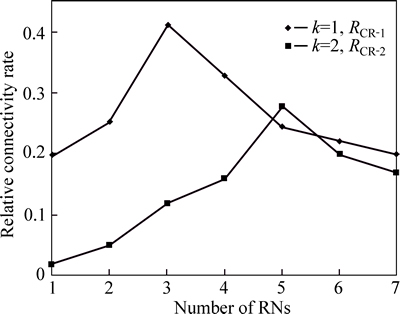
Fig. 8 Relative connectivity rate as a function of RNs’ number

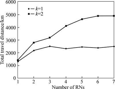
Fig. 9 Total travel distance as a function of RNs’ number

5.2.2 Performance comparison

We use the approach proposed [14] to realize the online movement control algorithm, and the metrics R_C-1, R_C-2 and D_TT for it are denoted by and  respectively. Then, we compare it with our proposed algorithm. The performance evaluation parameter is defined as the ratio between the metrics for our algorithm and the algorithm proposed in Ref. [14], i.e.,   and  We set w=12, m=5, and varied the ANs’ speed v to study the effects of network’s dynamic on the performance of the two algorithms. Figure 10 shows the performance ratio as a function of v for k=1 (Fig. 10(a)) and k=2 (Fig. 10(b)), respectively. The proposed algorithm [14] determines movement of RNs based on the current network topology; however, network topology may change to a new state when RNs arrive at their destinations in the highly-dynamic environment. Thanks to the topology estimation in our approach, our approach can significantly outperform that proposed in Ref. [14] in the highly-dynamic environment.

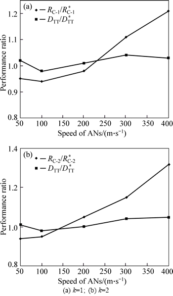
Fig. 10 Performance ratio as a function of ANs’ speed:

6 Conclusions

This work proposes an online algorithm for RNs’ movement control to maintain AANET a certain level connectivity during runing time and meanwhile make the total distance travelled by RNs minimal. The movement control problem is abstracted as MCFM problem, and a fast algorithm is proposed for it using the maximum weighted matching. Simulations show that the proposed algorithm outperforms other control approaches in the highly-dynamic environment and is of great potential to be applied in the highly-dynamic AANET to enhance the network’s connectivity.

References

[1] SAKHAEE E, JAMALIPOUR A. The global in-flight internet [J]. IEEE Journal on Selected Areas in Communications, 2006, 24(9): 1748-1757.

[2] SAKHAEE E, JAMALIPOUR A, KATO N. Aeronautical ad hoc networks [C]// Proceedings of the Wireless Communications and Networking Conference. Las Vegas, USA: IEEE, 2006: 246-251.

[3] KARRAS K, KYRITSIS T, AMIRFEIZ M. Aeronautical mobile ad hoc networks [C]// Proceedings of the 14th European Wireless Conference. Hong Kong: IEEE, 2008: 1-6.

[4] SCHNELL M, SCALISE S. NEWSKY—A concept for networking the sky for civil aeronautical communications [J]. Space Communications, 2008, 21(3): 157-166.

[5] KWAK K J, SAGDUYU Y, DENG J, YACKOSKI J, LI J. Airborne network evaluation: Challenges and high fidelity emulation solution [C]// Proceedings of The First ACM MobiHoc Workshop on Airborne Networks and Communications. Hilton Head, South Carolina, USA: ACM, 2012: 49-54.

[6] FALL K. A delay-tolerant network architecture for challenged internets [C]// Proceedings of ACM International Conference on the Applications, Technologies, Architectures, and Protocols for Computer Communication. Karlsruhe, Germany: ACM, 2003: 27-34.

[7] AZIZ A A, SEKERCIOGLU Y A, FITZPATRICK P, IVANOVICH M. A survey on distributed topology control techniques for extending the lifetime of battery powered wireless sensor networks [J]. IEEE Communications Surveys & Tutorials, 2013, 15(1): 121-144.

[8] NISHIYAMA H, NGO T, ANSARI N, KATO N. On minimizing the impact of mobility on topology control in mobile ad hoc networks [J]. IEEE Transactions on Wireless Communications, 2012, 11(3): 1158-1166.

[9] DAS S, LIU H, NAYAK A, STOJMENOVIC I. A localized algorithm for bi-connectivity of connected mobile robots [J]. Telecommunication Systems, 2009, 40(3): 129-140.

[10] NIGAM A, AGARWAL Y K. Optimal relay node placement in delay constrained wireless sensor network design [J]. European Journal of Operational Research, 2014, 233(1): 220-233.

[11] KASHYAP A, KHULLER S, SHAYMAN M. Relay placement for fault tolerance in wireless networks in higher dimensions [J]. Computational Geometry, 2011, 44(4): 206-215.

[12] ROHRER J P, JABBAR A, CETINKAYA E K, PERRINS E, STERBENZ J P. Highly-dynamic cross-layered aeronautical network architecture [J]. IEEE Transactions on Aerospace and Electronic System, 2011, 47(4): 2742–2765.

[13] OUYANG Jian, ZHUANG Yi, LIN Min, LIU Jia. Optimization of beamforming and path planning for UAV-assisted wireless relay networks [J]. Chinese Journal of Aeronautics, 2014, 27(2): 313-320.

[14] KASHYAP A, SHAYMAN M. Relay placement and movement control for realization of fault-tolerant ad hoc networks [C]// Proceedings of the 41st Annual Conference on Information Sciences and Systems. Baltimore, MD, USA: IEEE, 2007: 783-788.

[15] SENTURK I F, AKKAYA K, YILMAZ S. Relay placement for restoring connectivity in partitioned wireless sensor networks under limited information [J]. Ad Hoc Networks, 2014, 13: 487-503.

[16] LIN G H, XUE G. Steiner tree problem with minimum number of Steiner points and bounded edge-length [J]. Information Processing Letters, 1999, 69: 53-57.

[17] DEGENER B, FEKETE S P, KEMPKES B. A survey on relay placement with runtime and approximation guarantees [J]. Computer Science Review, 2011, 5(1): 57-68.

[18] CHERIYAN J, VEMPALA S, VETTA A. Approximation algorithms for minimum-cost k-vertex connected subgraphs [C]// Proceedings of the 34th Annual ACM Symposium on Theory of Computing. Montreal, Quebec, Canada: ACM, 2002: 306-312.

[19] WEST D B. Introduction to graph theory [M]. 2nd ed. London, UK: Pearson Education, 2000: 125-130.

[20] BREDIN J L, DEMAINE E D, HAJIAGHAYI M T, RUS D. Deploying sensor networks with guaranteed fault tolerance [J]. IEEE/ACM Transactions on Networking, 2010, 18(1): 216-228.

[21] OpenSim Ltd.. OMNET++ [EB/OL].[2015-01-30]. http://www.omnetpp.org.

[22] CAMP T, BOLENG J, DAVIES V. A survey of mobility models for ad hoc networks research [J]. Wireless Communications and Mobile Computing, 2002, 2(5): 483-502.

(Edited by DENG Lü-xiang)

Received date: 2015-01-30; Accepted date: 2015-05-19

Corresponding author: XIE Hong-wei, Professor, PhD; Tel: +86-731-84576311; E-mail: ljkjhk@126.com