J. Cent. South Univ. Technol. (2008) 15(s1): 307-310
DOI: 10.1007/s11771-008-369-0

Finite element analysis of fluid-structure interaction in buried liquid-conveying pipeline
ZHU Qing-jie(朱庆杰)1, CHEN Yan-hua(陈艳华)1, LIU Ting-quan(刘廷权)1, DAI Zhao-li(代兆立)2
(1. College of Civil Engineering and Architecture, Hebei Polytechnic University, Tangshan 063009, China;
2. Jidong Oilfield Company, China National Petroleum Corporation, Tangshan 063200, China)
Abstract: Long distance buried liquid-conveying pipeline is inevitable to cross faults and under earthquake action, it is necessary to calculate fluid-structure interaction(FSI) in finite element analysis under pipe-soil interaction. Under multi-action of site, fault movement and earthquake, finite element model of buried liquid-conveying pipeline for the calculation of fluid structure interaction was constructed through combinative application of ADINA-parasolid and ADINA-native modeling methods, and the direct computing method of two-way fluid-structure coupling was introduced. The methods of solid and fluid modeling were analyzed, pipe-soil friction was defined in solid model, and special flow assumption and fluid structure interface condition were defined in fluid model. Earthquake load, gravity and displacement of fault movement were applied, also model preferences. Finite element research on the damage of buried liquid-conveying pipeline was carried out through computing fluid-structure coupling. The influences of pipe-soil friction coefficient, fault-pipe angle, and liquid density on axial stress of pipeline were analyzed, and optimum parameters were proposed for the protection of buried liquid-conveying pipeline.
Key words: fluid-structure coupling; buried liquid-conveying pipeline; ADINA; finite element; faults; earthquake
1 Introduction
After transient analysis of fluid-structure systems was introduced by BATHE and HAHN[1] in 1978, theory on the fluid-structure coupling was developed rapidly. The influence of fluid-structure coupling on the axial vibration in liquid filling pipeline was investigated, and transfer matrixes were obtained with low frequency vibration[2-3]; nonlinear dynamic stability of liquid- conveying pipes was analyzed[4]. As basis of theory progress, more attention has been paid on finite element analysis. Finite element equations of liquid-structure coupling for liquid-conveying were obtained[5]; a finite element formula for the fully coupled dynamic equations of motion including the effect of fluid- structure interaction was introduced and applied to a pipeline system[6]. It is inevitable to cross faults for long distance buried liquid-conveying pipeline. Therefore, the damage of buried pipeline is serious under earthquake action. For example, Tangshan earthquake in 1976, made the total water supply pipelines destroyed, and more than 10 kt crude oil lost. In recent years, earthquakes in China, such as Dayao earthquake of Yunnan Province in 2003, Dongwu earthquake of Inner Mongolia AUT.REG. in 2004, Yanjin earthquake of Yunnan Province in 2006, Puer earthquake of Yunnan Province in 2007, which made lots of buried pipeline damaged, especially Wenchuan earthquake of Sichuan Province in 2008. Therefore, influence of site and fault movement on the buried pipeline damage is another main problem[7-8]. In this work, fluid-structure interaction was combined with fault and site action, and fluid-structure coupling was calculated under pipe-soil (site) interaction. Multi- actions of earthquake, fault movement, and gravity were applied, and influences of pipe-soil friction, fault, and liquid density on the axial stress of pipelines were analyzed.
2 Fluid-structure interaction model
In fluid-structure interaction analysis, fluid forces are applied to the solid, and the solid deformation changes the fluid domain. The computational domain is divided into the fluid domain and solid domain, and fluid-structure interaction occurs along the interface of the two domains. For most interaction problems, a fluid model and a solid model are defined respectively. A fluid-structure interaction model for buried liquid- conveying pipeline is illustrated in Fig.1. The fluid model is defined in the fluid domain with boundary conditions, such as velocity at the inlet and the outlet, and more important, the fluid structure interface condition. The solid model is defined in the structural
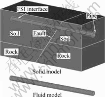
Fig.1 Model of fluid-structure interaction
domain, where shell surfaces of pipe are the fluid structure interfaces, and the site contact with pipe through pipe-soil friction.
The typical task of fluid-structure analysis is to obtain the fluid and structure response through the coupled solution. The structural model is based on a Lagrangian coordinate system, and the displacements are primarily unknown. Because the fluid-structure interface is deformable, the fluid model must be based on an arbitrary-Lagrangian-Eulerian coordinate system. Therefore, the solution variables of the fluid flow include not only the usual fluid variables, such as pressure and velocity, but also displacements.
Completely different elements and meshes can be used in fluid and solid models. The nodal positions of the two models are not therefore generally the same on the fluid-structure interface. The fluid nodal displacements are interpolated using the adjacent solid nodal displacements. Similarly, the fluid stress at solid node is interpolated using the fluid stresses at adjacent fluid nodes, while the stresses at solid nodes equal the fluid stresses at fluid nodes. The fluid solution variables and the solid solution variables at the numbered nodes are therefore eventually coupled.
3 Direct computing of two-way coupling
The fundamental conditions applied to the fluid-structure interfaces are the kinematic condition and the dynamic condition:
df=ds (1)
n?σf=n?σs (2)
where df and ds are respectively the fluid and solid displacements; σf and σs are respectively the fluid and solid stresses.
The fluid velocity condition is resulted from the kinematic condition:
nν=nds (no-slip) (3)
nν=nd (slip) (4)
The fluid nodal positions on the fluid-structure interfaces are determined by the kinematic conditions. The displacements of the other fluid nodes are determined automatically by the program to preserve the initial mesh quality. According to the dynamic conditions, on the other hand, the fluid traction is integrated into fluid force along fluid-structure interfaces and exerted onto the structure nodes.
 (5)
(5)
where hd is the virtual quantity of solid displacement.
The solution vector of the coupled system is
X=(Xf, Xs) (6)
where Xf and Xs are the fluid and solid solution vectors defined at fluid and solid nodes, respectively. Thus,
ds=ds(Xs) (7)
df=σf(Xf) (8)
The finite element equations of the fluid- structure couple system can be expressed as
 (9)
(9)
where Ff and Fs are finite element equations. Note that the decoupled fluid and solid equations can be represented by Ff[Xf, 0]=0 and Fs[Xs, 0]=0 respectively.
For many coupled problems, the fluid traction affects the structural deformations, and the solid displacement affects the flow pattern. This fact is the reason for performing fluid-structure interaction analysis. This type of analysis is called two-way coupling. Because the fluid equations are always nonlinear, Eqn.(9) is a nonlinear system regardless of the solid model whether it is linear or not, and an iteration procedure must be used to obtain the solution at a specific time. Criteria, either stress or displacement, or both of these, are used to check for convergence of the iterations.
There are two solution methods, direct computing and iterative computing methods. The computing speed of direct method in general is faster than that of the iterative method in two-way couplings. It is suitable for small to medium problems, and also good for transient analysis. Direct computing method of two-way coupling is also called the simultaneous solution method. In this direct solution method, the fluid and solid solution variables are fully coupled. The equations of fluid and solid are combined and treated in one system. Therefore, they are linearized in a matrix system. This matrix system can be written as
 (10)
(10)
Xk+1=Xk+ΔXk (11)
For example, when the Newton-Raphson method is used, then

 (12)
(12)

 (13)
(13)
 (14)
(14)
 (15)
(15)
where λd (0<λd≤1) is displacement relaxation factor, and λσ (0<λσ≤1) is stress relaxation factor.
The computational procedure can be summarized as follows. In order to obtain the solution at time t+Δt with the initial solution guess X0=Xt, for iterations k=1, 2, …, the equilibrium iteration procedure is performed to obtain the Xt+Δt.
4 Finite element modeling
The main problem is the definition of solid models and fluid models.
4.1 Defining solid models
Solid model geometry is constructed in ADINA- structure solver, site model is established with ADINA- parasolid geometry modeling, and pipe model geometry is established with ADINA-native geometry modeling. The surfaces of the pipe are modeled with 9-node shell elements. More important, fluid-structure boundaries must be defined, and the two surfaces of pipe shell are fluid-structure interface.
One most important problem is the contact between site and pipe, which is defined as pipe-soil friction. ADINA has a general Coulomb type friction model, where the friction coefficient m? can be a constant, or a function of the normal contact tractions, or calculated based on a user-supplied friction law. The basic friction model can be written as,
Tt=μTn (16)
where μ is a specified constant; Tt is the maximum tangential traction, and Tn is the normal traction.
Loads include gravity load, displacement load of fault movement, and load of earthquake wave. The earthquake load is nonlinear, and shown in Fig.2.
In the direct computing method, the fluid flow
model controls the time steps. Hence the same control parameters specified in the solid solver are ignored in the solution procedure. However, time functions defined in the solid model must cover the time range of the
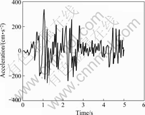
Fig.2 Time function of earthquake wave
computation. The parameters that control the convergence of the coupled system are also processed in the fluid model. These parameters are the stress and displacement tolerances, relaxation factors, convergence criteria, etc.
4.2 Defining fluid model
The fluid element is defined as 3D fluid element, and velocity load is applied. The relative tolerance for degrees of freedom is set to 0.01. The type of fluid-structure interface is surface, and slip condition is selected. There are four liquid materials; material properties include density and viscosity.
After the modeling of solid and fluid models, save them as solid and fluid files. Run ADINA- FSI and select both solid and fluid files to obtain results.
5 Results analysis
Fig.3 is axial stress―time curve affected by pipe- soil friction coefficient. It can be found that axial stress is minimum when friction coefficient is 0.4, which means that 0.4 is the optimum value.
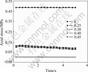
Fig.3 Axial stress affected by friction coefficient
Three fault-pipe angles are calculated, namely, are 45?, 60? and 90? (shown as Fig.4). It can be found that axial stress is the minimum when fault-pipe angle is 60?, which means that 60? is the optimal value of fault-pipe angles for buried pipeline protection.
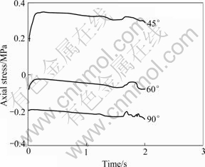
Fig.4 Axial stress affected by fault-pipe angle
Fig.5 shows the maximum of axial stress affected by liquid density. Axial stress decreases as the liquid density becomes smaller and smaller. It means that more protection should be done for heavy liquid.
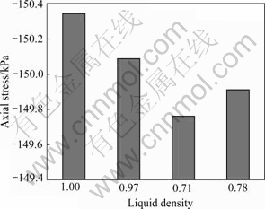
Fig.5 Influence of fluid density on axial stress
6 Conclusions
By finite element analysis, some conclusions are obtained as follows.
1) Earthquake and faults loads are applied to solid model of buried liquid-conveying pipeline, stress and displacement distribution of buried pipeline can be calculated through computing of fluid-structure coupling under pipe-soil interaction, and the influence of liquid can be analyzed.
2) Pipe-soil friction and fault movement are two main factors, which control the damage of buried pipeline. When friction coefficient is 0.4, axial stress is the minimum. This gives a way to decrease the damage of buried pipeline through the selection or changing of backfill soil properties. Axial stress is the minimum when fault-pipe angle is 60?. Therefore, 60? is the optimal value of fault-pipe angles if pipeline has to cross faults.
3) The heavier the liquid density, the bigger the axial stress. Therefore, more protection should be done for heavy liquid conveying buried pipeline.
References
[1] BATHE K J, HAHN W. On transient analysis of fluid-structure systems [J]. J Computers and Structures, 1978, 10(2): 383-391.
[2] ZHANG Zhi-yong, SHEN Rong-ying. Fluid-structure interaction of the straight liquid-filled piping system [J]. Journal of Vibration Engineering, 2000, 13(3): 455-461. (in Chinese)
[3] ZHANG Zhi-yong, SHEN Rong-ying, WANG Qiang. The model analysis of the liquid-filled pipe system [J]. Chinese Journal of Solid Mechanics, 2001, 22(2): 143-149. (in Chinese)
[4] ZHANG Li-xiang, HUANG Wen-hu. Analysis of nonlinear dynamic stability of liquid-conveying pipes [J]. Applied Mathematics and Mechanics, 2002, 23(9): 951-960. (in Chinese)
[5] WANG Shi-zhong, YU Shi-sheng, ZHAO Yang. Solid-liquid coupling characteristics of fluid-conveying pipes [J]. Journal of Harbin Institute Technology, 2002, 34(2): 141-144. (in Chinese)
[6] SREEJITH B, JAYARAJ K, GANESAN N, et al. Finite element analysis of fluid-structure interaction in pipeline systems [J]. Nuclear Engineering and Design, 2004, 227(3): 313-322.
[7] ZHU Qing-jie, LIU Ying-li, JIANG Lu-zhen, et al. Analysis of buried pipeline damage affected by pipe-soil friction and pipe radius [J]. Earthquake Engineering and Engineering Vibration, 2006, 26(3): 197-199. (in Chinese)
[8] DIMITRIOS K K, GEORGE D B, GEORGE P K. Stress analysis of buried steel pipelines at strike-slip fault crossings [J]. Soil Dynamics and Earthquake Engineering, 2007, 27(3): 200-211.
(Edited by CHEN Wei-ping)
Foundation item: Project(50678059) supported by the National Natural Science Foundation of China
Received date: 2008-06-25; Accepted date: 2008-08-05
Corresponding author: ZHU Qing-jie, Professor, PhD; Tel: +86-315-2616969, +86-13932521086; E-mail: qjzhu@heut.edu.cn

