J. Cent. South Univ. Technol. (2011) 18: 2001-2008

DOI: 10.1007/s11771-011-0934-9

Modified Wiener method in diffusion weighted image denoising

YI San-li(易三莉)¹, CHEN Zhen-cheng(陈真诚)², LING Hong-li(林红利)¹

1. Earth Science and Information Institute of Physics, Central South University, Changsha 410083, China;

2. Life and Environment Institute, Guilin University of Electronic Technology, Guilin 541004, China

? Central South University Press and Springer-Verlag Berlin Heidelberg 2011

Abstract: To denoise the diffusion weighted images (DWIs) featured as multi-boundary, which was very important for the calculation of accurate DTIs (diffusion tensor magnetic resonance imaging), a modified Wiener filter was proposed. Through analyzing the widely accepted adaptive Wiener filter in image denoising fields, which suffered from annoying noise around the edges of DWIs and in turn greatly affected the denoising effect of DWIs, a local-shift method capable of overcoming the defect of the adaptive Wiener filter was proposed to help better denoising DWIs and the modified Wiener filter was constructed accordingly. To verify the denoising effect of the proposed method, the modified Wiener filter and adaptive Wiener filter were performed on the noisy DWI data, respectively, and the results of different methods were analyzed in detail and put into comparison. The experimental data show that, with the modified Wiener method, more satisfactory results such as lower non-positive tensor percentage and lower mean square errors of the fractional anisotropy map and trace map are obtained than those with the adaptive Wiener method, which in turn helps to produce more accurate DTIs.

Key words: diffusion weighted image (DWI); diffusion tensor image (DTI); local-shift method; modified Wiener filter

1 Introduction

The appearance of the diffusion tensor magnetic resonance imaging (DT-MRI) technique is a great progress in the medical image fields. The DT-MRI, commonly known as diffusion tensor imaging (DTI), is the only clinical noninvasive method of imaging the white matter of the brain in vivo. The most important utility of DTI is that it provides a way of identifying nerve fiber tracts. Diffusion tensor image can be derived from the diffusion weighted images. The noise from the diffusion weighted image (DWI) is particularly harmful to fiber tracking because it will produce error in the estimation of the tensor and consequently lead to the deflection of the fiber path direction, and such harmful impact accumulates during the tracking process [1]. Therefore, a more effective denoising method is essential to DTI data.

The denoising method applied to DTI can be roughly divided into two categories. One category is to perform the denoising process in DWIs prior to the determination of the DTI. Many experts have engaged in the study of denoising DWIs. In 2005, DING et al [2] proposed anisotropic smoothing approaches based on stochastic relaxation. In 2006, SAURAV [3] presented a posteriori estimation technique that directly operated on the diffusion weighted images. McGRAW et al [4] used a weighted TV-norm method to smooth the diffusion-weighted data. In 2009, MARTIN et al [5] proposed sequential anisotropic Wiener filtering method. Another category is to perform the denoising process posterior for the determination of DTI, i.e. the DTI is directly computed from the raw noisy DWIs and then denoised, which has been applied by many researchers such as CASTANO et al [6], XAVIER et al [7] and PIERRE [8]. Although the second category has been widely adopted, it is not considered quite reasonable, just as DEREK and BASSER [9] has reported: the background noise present in the DWI produced an underestimation (bias) of indices of diffusion anisotropy which was not possible to be corrected once the DTI data were determined. Therefore, the first category will be adopted in this work, i.e. to perform the denoising process on the DWI prior to the computation of the diffusion tensor image.

As diffusion weighted images are affected by several artifacts and noise from different channels, the random variation of these quantities complicates the analysis and interpretation of DTI data [10]. In order to enhance the reliability of the DTI data, it is essential to use a more effective method to minimize or eliminate the noise in the DWI. Adaptive Wiener filter is a widely used and effective denoising method in the image denoising field. The theory of adaptive Wiener filter was originally proposed by LEE [11], which is successful in the sense that it effectively removes noise while preserving important image edges. Although LEE’s approach has been widely applied in many researches, it still suffers from annoying noise around edges due to the assumption that all samples within a local window are from the same ensemble [12]. With a view to resolving the problem of LEE’s approach, some researches have been conducted by many other scholars to improve LEE’s filter. DARWIN [12] proposed the adaptive weighted Wiener method with which the Wiener filter could be adaptively weighted. In 1993, MEHMET [13] proposed the method of adaptive weighted averaging (AWA). Later, JIN et al [14] combined wavelet Wiener method with AWA. Based on the above mentioned research, in this work, a modified Wiener method is proposed for the purpose of better denoising the DWI.

2 Adaptive Wiener method

2.1 Adaptive Wiener filter

The Wiener filter is the optimum linear filter in the sense of mean square error. Its definition is presented as [15]

                                                        (1)

where σ²(x, y) is the signal variance, and  is the noise variance.

The DWI is denoised by the Wiener filter as

                        (2)

where f(x, y) is the DWI, g(x, y) is the output of Wiener filter, and  is the mean value of f(x, y).

According to LEE’s method, the spatial adaptive Wiener filter can be calculated locally by using the local statistics which can be obtained through calculating over a uniform moving average window with size of (2r+1)× (2s+1):

                 (3)

and

(4)

where  is the local mean value, σ²(x, y) is the local variance, and f (p, q) is the neighbor element of    f (x, y) within the average window.

2.2 Analysis of adaptive Wiener filter

The adaptive Wiener filter is based on the assumption that the stationary is locally satisfied. The local signal variance of the different elements in an image is different, and different values of the local variance in the image present different change extents of the signal. A field with relative smooth signal change is a homogeneous region, where the local variance is low. A field with relative sharp signal change is an inhomogeneous region, where the local variance is large [5].

In Eq.(1), as the local variance σ²(x, y) varies with the spatial variation, the adaptive Wiener filter calculated from the local variance varies accordingly. When the local variance is relatively large, the value of filter w converges towards 1. When the local variance is relatively low, the value of filter w converges towards 0.

Equation (2) can be rearranged as

                             (5)

From Eq.(5), it can be observed that the value of filtered image g(x, y) is actually determined by the value of w. When w is close to 0, the result of Eq.(5) is mainly determined by the second part of the right side, i.e.  This means that the result of the filter is the average of the local neighbors of f(x, y). When w is close to 1, the result of Eq.(5) is mainly determined by the first part of the right side, i.e.  This means that the original data would remain nearly untouched.

It is well known that the change of the signal in an image is always sharp in the boundary, which means that the boundary signal is in the inhomogeneous region and its variance is very large. From the above analysis, it is noticed that because the large variance at the boundary causes the value of Wiener filter to be close to 1, the adaptive Wiener filter leaves the original noisy signal nearly untouched, i.e. the output of the filter is actually still noisy. Such results are certainly not quite satisfactory. As for such results, KUAN has explained [12] that it is because the adaptive Wiener filter is based on the assumption that all samples within a local window are from the same ensemble, and this assumption is invalidated if there is a sharp edge within the window.

According to Eq.(4), the local variance σ²(x, y) of a point f(x, y) in the DWI reflects the signal’s change of the neighbor element f(p, q) within the local average window. If σ²(x, y) is small, it means that the change of f(p, q) is small, and the elements within the local average window including f(x, y) are more likely to belong to the same ensemble; if σ²(x, y) is large, then the change of the f(p, q) is sharp, and the elements including f(x, y) are more likely to belong to different ensembles. For the boundary signal, because the change of its neighbor elements is very large, the local statistics such as local variance σ²(x, y) and local mean  figured out from the local elements belonging to different ensembles cannot accurately express the real statistics of the boundary signal f(x, y). Consequently in Eq.(8), the Wiener filter calculated from such inaccurate statistics will not be reliable. Therefore, a local-shift method with which more accurate local statistics can be figured out will be proposed and discussed.

3 Modified Wiener filter

In DWI, which has multi-boundary in nature, and from which DTI is calculated, accurate boundary signals are particularly important for the calculation of diffusion signals on which the tracking of the possibly existing fibers in boundary regions are relied. Therefore, to preserve the original noisy boundary signal in adaptive Wiener filter will lead to inaccurate diffusion tensor with inaccurate eigenvalues and eigenvectors and thus affect the fiber tracking. In this section, the local-shift method is proposed to obtain more reliable boundary signals, and a modified Wiener filter based on this method is constructed accordingly.

3.1 Local-shift method

According to the above analysis, for a boundary signal f(x, y), as the neighbor elements in its local average window (in this work, the size of local average window is set as 3×3, i.e. the values of r and s in Eq.(3) are 1, so the number of neighbor elements is 8) belong to different ensembles, the data calculated from such local neighbor elements are not accurate. As the local elements belonging to the same ensemble have the same statistics such as the same variance and the same mean value, through finding out the local elements belonging to the same ensemble as the boundary signal f(x, y), accurate statistics can be obtained.

In Fig.1, Ω₀ denotes the local dataset within the local average window which is centered on the boundary signal f(x, y). Ω_i (i1, 2, …, 8) denotes the local dataset centered on the neighbor element of f(x, y), i.e. centered on f(p, q). Figure 1 shows that the local dataset Ω_i of each neighbor element f(p, q) includes the boundary signal f(x, y).

Through comparing the local variance σ²(p, q) of each neighbor element f(p, q), the local dataset, of which all the elements including the boundary signal f(x, y) belong to the same ensemble, can be found. Such dataset is figured out through the following equation:

                                                 (6)

where Ω_k is the local dataset of neighbor element with minimal local variance, σ²(p, q) is the local variance of  f(p, q) which is the neighbor element of the boundary signal f(x, y). Based on the above analysis, the boundary signal f(x, y) is more likely to belong to the same ensemble as the dataset Ω_k with the minimal local variance. Then, to get more reliable local variance and local mean value of boundary signal f(x, y), the local dataset based on which the local statistics of f(x, y) are figured out is shifted from Ω₀ to Ω_k. The new local statistics of f(x, y) are  and  (called as local-shift variance and local-shift mean, respectively, in this work), so the modified local-shift Wiener filter w_k at the boundary is shifted accordingly and it can be defined as

                                                      (7)

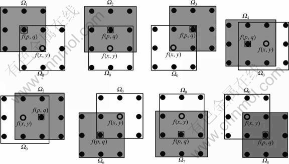
Fig.1 Local dataset Ω_i (i1, 2, …, 8) centered on neighbor element f(p, q) of f(x, y)

3.2 Modified Wiener filter

While in homogeneous region, the change of the signal is relatively smooth, and the output of the adaptive Wiener filter is reliable. Therefore, a modified Wiener filter, which adopts different denoising methods in different regions, is constructed.

The modified Wiener filter is divided into two parts. One is applied in the low variance region, i.e. homogeneous region, and the other is applied in the large variance region i.e. inhomogeneous region. In order to detect different regions of DWI, a threshold parameter t of the image is used. The value of t is defined as

                                 (8)

where  is the mean value of the local variances of DWI,  is the maximum value of the local variances of DWI, and λ is the regularization parameter which is set between 0 and 1.

When the local variance of the image element f(x, y), σ²(x, y), is lower than t, it means that the signal f(x, y) is in low variance region i.e. homogeneous region. When σ²(x, y) is larger than t, it means that f(x, y) is in inhomogeneous region. In inhomogeneous region, the filter is modified to get more reliable result; while in homogeneous region, LEE’s adaptive Wiener filter is still used to denoise the data. The definition of modified Wiener filter is

(9)

where g(x, y) is the output of modified Wiener filter,   f(x, y) is the original noisy image,  is the local mean of f(x, y), w represents the adaptive Wiener filter,  is the local-shift mean of f(x, y), and w_k is the local-shift Wiener filter figured out from Eq.(7).

According to Eq.(9), when σ²(x, y)≤t, the adaptive Wiener filter w is used to process the original noisy image; when σ²(x, y)>t, the output of adaptive Wiener filter is not reliable, and the local-shift Wiener filter w_k should be adopted.

4 Experiment and discussion

Diffusion tensor can be represented as a diffusion ellipsoid [16]. The eigenvectors of the diffusion tensor provide directions for the axis of ellipsoid, and their corresponding eigenvalues give the length of the axis of ellipsoid. The most usually used diffusion indexes of DTI are the fractional anisotropy (FA) and the Trace, which can be figured out from Ref.[17]. In this section, denoising experiments were carried out on synthetic and real diffusion weighted images. The modified Wiener filter was applied to DWIs and its results were compared with those obtained by applying adaptive Wiener filter.

4.1 Synthetic tensor data

A 16×16 synthetic diffusion tensor image, generated from six diffusion weighted images and one baseline image, is shown in Fig.2(a). The gradient direction corresponding with the DWIs was the commonly used direction, i.e. (1, 1, 0), (0, 1, 1), (1, 0, 1), (0, 1, -1),    (1, -1, 0) and (-1, 0, 1), as that shown in Ref.[18]. In Fig.2, the boundaries of the image were constructed by the tensors with different FA values. The FA value of the tensor of the frame was set as 0.5, and the FA value of other tensor was 0.7. To compare different denoising results brought about by different methods, firstly, Gaussian noise with its SNR (signal to noise ratio) set as 10 was added to the 6 DWIs, and then a noisy DTI was calculated from the noisy DWIs, as shown in Fig.2(b). Secondly, the noisy DWIs were smoothed with the modified Wiener method (MW) and adaptive Wiener method (AW), respectively. Figure 2(c) shows the DTI computed from the DWIs denoised by adaptive Wiener method and Fig.2(d) the DTI computed from the DWIs denoised by modified Wiener method. From the four DTIs of Fig.2, it is obviously shown that the performance of the modified Wiener method is better than that of the adaptive Wiener method due to its more accurate boundary recovery. The boundaries in Fig.2(d) are more accurate than those in Fig.2(c).

The deviation of DWI data caused by noise will make the tensor computed from these noisy DWI data become non-positive, which is known as non-positive tensor (NPT). The number of such non-positive tensors in the DTI can be reduced through denoising the DWIs. Different approaches produce different effects on the deviation-correction. In order to quantitatively compare the performance of the modified Wiener method with that of the adaptive Wiener method, it is proposed to compare the different percentages of non-positive tensor of DTI figured out with these two approaches. The DTI illustrated here was computed from six 256×256-sized  DWIs (shown in s1-s6 of Fig.3), with the same size as the DWIs. The baseline image s0 of this DTI was set as a fixed value of 1.0, and had the same size as the DWIs. The distribution of the tensors with different FA values in the image was the same as Fig.2, where the FA value of the tensor of the frames was 0.5, that of the rest tensor was 0.7, and the difference was that the number of frames in the tensor image was set as 20. The Gaussian noise with changing SNR (ranging from 5 to 30 with step-size of 5) was added to each of the DWI (s1-s6), and then the noisy DWIs were smoothed with different methods under different levels of SNR. Figure 3 (n1-n6) presents the noisy DWIs with SNR of 10. Table 1 lists the comparison between the denoised results of the modified Wiener method and those of the adaptive Wiener method, and the comparison between the results of pre-processing (the DWI image denoising process carried out prior to the determination of the DTI) and that of post-processing (the DWI image denoising process carried out after the determination of the DTI). The percentage of NPT in the DTI denoised with the modified Wiener method is lower than that denoised with the adaptive Wiener method, and the NPT percentage resulting from pre-processing is also lower than that from post-processing, which shows that with the modified Wiener approach, the denoising process performed on the DWIs before determination of DTI provides more accurate result.

Fig.2 Synthetic tensor images: (a) Original synthetic tensor image; (b) Noisy tensor image with SNR of 10; (c) Tensor image resulting from application of adaptive Wiener filter (AW); (d) Tensor image resulting from application of modified Wiener filter (MW)

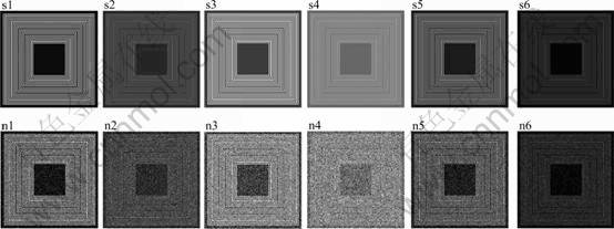
Fig.3 Synthetic diffusion weighted images with size of 256×256 and number inside frames of DWI set as 20: (s1-s6) Original synthetic DWIs; (n1-n6) Noisy DWIs with SNR of 10 and Gaussian noise being added

4.2 Synthetic FA and Trace data

To make a further analysis of the results obtained with different denoising methods, the indexes of DTI such as FA map and Trace map was analyzed. The mean squared error (MSE) between the original noisy FA map (and Trace map) and the denoised FA map (and Trace map) is calculated. Figure 4 presents the functions of the MSE from different denoising methods, varying with increasing SNR (ranging from 5 to 40 with step-size set as 5). Figure 4(a) presents a comparison of the MSE on FA from the two different methods varying with increasing SNR; Fig.4(b) presents a comparison of the MSE on Trace from the two different methods varying with increasing SNR. Figure 4 reveals that the modified Wiener method achieves smaller MSE at all levels of SNR. Moreover, this method performs better than the adaptive Wiener method at lower level of SNR.

To compare the denoising results of the different methods on the multi-boundary DWI, the MSE changing with increasing the number of boundaries under a given SNR were calculated. The Gaussian noise with SNR set as 20 was added to the DWIs, s1-s6 in Fig.3. The above analysis shows that the amounts of boundaries increase with increasing the frame number. Figure 5 shows the comparison of the results obtained from different denoising methods under the increasing numbers of frames (ranging from 4 to 24 with step-size of 4). Figure 5(a) plots a comparison of the MSE on FA map resulting from the application of the two different denoising methods, expressed as the function of the increasing frames. Figure 5(b) plots a comparison of the MSE on Trace map resulting from the application of the two different denoising methods, expressed as the function of the increasing frames. According to Fig.5, the modified Wiener filter is more suitable to the multi-boundary DWIs. With the number of boundaries increasing, the denoising effect of the modified Wiener becomes increasingly better than that of the adaptive Wiener method because of the lower MSE both on FA map and Trace map of DTI.

4.3 Real diffusion MRI data

The real diffusion weighted images were acquired on a 1.5 T General Electric MRI system of a normal volunteer. The sequence parameters were chosen as TR 12 000 ms, TE 107 ms, b=1 000 s/mm². The size of the acquired image was 256×256 and the voxel size was    1 mm × 1 mm × 4 mm. A 13 direction gradients scheme was used and acquisitions were repeated five times for each direction. Both modified Wiener filter and adaptive Wiener filter were applied to denoising these DWIs, and their respective resulting FA images are shown in Fig.6. Figure 6(a) shows the FA image computed from the original DWIs, Fig.6(b) shows the FA image from the DWIs denoised by the adaptive Wiener method, and Fig.6(c) shows the FA image from DWIs denoised by the modified Wiener method. It can be seen from Fig.6 that DWIs denoised with the modified Wiener method preserves white matter structures well, with less blurring effect than the DWIs denoised with the adaptive Wiener method. From this result, the same conclusion as that drawn in synthetic data can be reached that more accurate data can be acquired with the modified Wiener method which is suitable for multi-boundary diffusion weighted images.

Table 1 Different percentages of NPT resulting from application of different denoising methods under different levels of SNR (%)

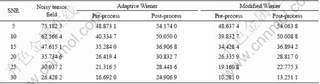
Fig.4 Function of MSE under different noise levels (SNR ranging from 5 to 40 with step-size set as 5, and inside synthetic DWIs number of frames set as 20): (a) Comparison of MSE on fractional anisotropy; (b) Comparison of MSE on Trace

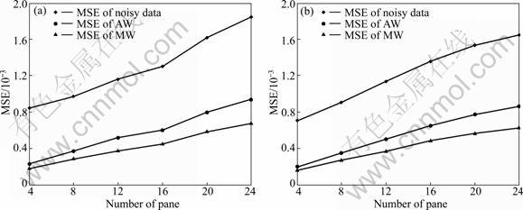
Fig.5 Function of MSE under different edge numbers (number of frames in synthetic DWIs ranging from 4 to 24 with step-size of 4, and SNR of dataset set as 20): (a) Comparison of MSE on fractional anisotropy; (b) Comparison of MSE on Trace

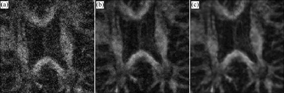
Fig.6 FA images from real DWIs denoised by different methods: (a) FA image computed from original DWIs; (b) FA image from processed DWIs with adaptive Wiener method; (c) FA image from processed DWIs with modified Wiener method

5 Conclusions

1) The modified Wiener filter capable of overcoming the defect of the adaptive Wiener filter performs more effective than adaptive Wiener filter in denoising DTIs. And the denoising process conducted on the DWIs before the determination of DTI leads to more accurate DTIs. The experimental data show that the percentage of NPT in the DTI denoised with the modified Wiener method is lower than that denoised with the adaptive Wiener method, and the NPT percentage resulting from pre-processing is also lower than that from post-processing, which shows that with the modified Wiener approach, the denoising process carried out on the DWIs before the determination of DTI provides more accurate result.

2) The modified Wiener filter based on the local-shift wiener method and capable of getting more accurate boundary signals are especially suitable for denoising multi-boundary images. The comparison of applying the adaptive Wiener filter and the modified Wiener filter to the synthetic FA and Trace data, respectively, shows that with increasing the number of the boundaries, the modified Wiener filter still performs well, while the other filter performs worse.

3) The modified Wiener method is a more effective method to denoise DTIs. A lower non-positive tensor percentage and lower mean square errors of the FA map and Trace map are obtained by applying the modified Wiener method than by the adaptive Wiener method, which leads to more accurate DTIs.

References

[1] Arabinda M, LU Yong-gang, MENG Jing-jing, Adam W A, Ding Zhao-hua. Unified framework for anisotropic interpolation and smoothing of diffusion tensor images [J]. Neuro Image, 2006, 31(4): 1525-1535.

[2] Ding Zhao-hua, John G G, Adam W A. Reduction of noise in diffusion tensor images using anisotropic smoothing [J]. Magnetic Resonnance in Medicine 2005, 53(2): 485-490.

[3] Saurav B, Thomas F, Ross W. Rician noise removal in diffusion tensor MRI [J]. Medical Image Computing and Computer- Assisted Intervention, 2006, 9(1): 117-125.

[4] McGraw T, Vermuri B C, Chen Y, RAO M, MARECI T. DT-MRI denoising and neuronal fiber tracking [J]. Medical Image Analysis, 2004, 8(2): 95-111.

[5] Martin F M, Munoz M E, CAMMOUN L. Sequential anisotropic multichannel Wiener filtering with Rician bias correction applied to 3D regularization of DWI data [J]. Medical Image Analysis, 2009, 13(1): 19-35.

[6] Castano M C A, Lenglet C, Deriche R. A Riemannian approach to anisotropic filtering of tensor fields [J]. Signal Processing, 2007, 87(2): 263-276.

[7] Xavier P, Piere F, Nicolas A. A riemannian framework for tensor computing [J]. International Journal of Computer Vision, 2006, 66(1): 41-66.

[8] Pierre F, Vincent A, Xavier P, Nicholas A. Clinical DT-MRI estimation, smoothing and fiber tracking with log-Euclidean metrics [J]. IEEE Transactions on Medical Imaging, 2007, 26(11): 1472-1482.

[9] Derek K J, Basser P J. Squashing peanuts and smashing pumpkins: How noise distorts diffusion-weighted MR data [J]. Magnetic Resonnance in Medicine, 2004, 52(5): 979-993.

[10] Adam W A. Theoretical analysis of the effects of noise on diffusion tensor imaging [J]. Magnetic Resonnance in Medicine, 2001, 46(6): 1174-1188.

[11] Lee J S. Digital image enhancement and noise filtering by use of local statistics [J]. IEEE Transactions on Pattern Analysis and Machine Intelligence, 1980, PAMI-2(2): 165-168.

[12] Darwin T K, Alexander A S, TIMOTHY C S, PIERRE C. Adaptive noise smoothing filter for images with signal-dependent noise [J]. IEEE Trans PAMI, 1985, 7(2): 165-177.

[13] Mehmet K O, Ibrahim S M, Mruat T A. Adaptive motion compensated filtering of noisy image sequences [J]. IEEE Trans CSVT, 1993, 3(4): 277-289.

[14] Jin F, Fieguth P, JERNIGAN E. Adaptive wiener filtering of noisy images and image sequences [J]. Proceedings 2003 International conference on Image Processing, 2003, 2(3): 349-352.

[15] Simon S H. Adaptive filter theory [M]. 4th Ed. ZHENG Bao-yu, Tr. Beijing: Publishing House of Electronics Industry, 2002, 70-92.

[16] Aziz M U, Peter C M V Z. Orientation-independent diffusion imaging without tensor diagonalization: Anisotropy definitions based on physical attributes of the diffusion ellipsoid [J]. Journal of Magnetic Resonance Imaging, 1999, 9(6): 804-813.

[17] Basser P J, Carlo P. Microstructural and physiological features of tissues elucidated by quantitative-diffusion-tensor MRI [J]. Journal of Magnetic Resonance Series B, 1996, 111(3): 209-219.

[18] Westin C F, Maier S E, Mamata H, NABAVI A, JOLESZ F A, KIKINIS R. Processing and visualization for diffusion tensor MRI [J]. Medical Image Analysis, 2002, 6(2): 93-108.

(Edited by YANG Bing)

Foundation item: Project(2009AA04Z214) supported by the National High Technology Research and Development Program of China; Project(07JJ6133) supported by the Natural Science Foundation of Hunan Province, China

Received date: 2010-10-13; Accepted date: 2010-12-30

Corresponding author: YI San-li, PhD Candidate, Tel: +86-13507481826; E-mail: litch2004@sina.com