J. Cent. South Univ. (2016) 23: 2735-2746

DOI: 10.1007/s11771-016-3335-2

Detached-eddy simulation of flow around high-speed train on a bridge under cross winds

CHEN Jing-wen(陈敬文)^{1, 2}, GAO Guang-jun(高广军)^{1, 2}, ZHU Chun-li(朱春丽)^{1, 2}

1. School of Traffic & Transportation Engineering, Central South University, Changsha 410075, China;

2. Key Laboratory of Traffic Safety on the Track of Ministry of Education (Central South University), Changsha 410075, China

Central South University Press and Springer-Verlag Berlin Heidelberg 2016

Abstract: In order to describe an investigation of the flow around high-speed train on a bridge under cross winds using detached-eddy simulation (DES), a 1/8th scale model of a three-car high-speed train and a typical bridge model are employed, Numerical wind tunnel technology based on computational fluid dynamics (CFD) is used, and the CFD models are set as stationary models. The Reynolds number of the flow, based on the inflow velocity and the height of the vehicle, is 1.9×10⁶. The computations are conducted under three cases, train on the windward track on the bridge (WWC), train on the leeward track on the bridge (LWC) and train on the flat ground (FGC). Commercial software FLUENT is used and the mesh sensitivity research is carried out by three different grids: coarse, medium and fine. Results show that compared with FGC case, the side force coefficients of the head cars for the WWC and LWC cases increases by 14% and 29%, respectively; the coefficients of middle cars for the WWC and LWC increase by 32% and 10%, respectively; and that of the tail car increases by 45% for the WWC whereas decreases by 2% for the LWC case. The most notable thing is that the side force and the rolling moment of the head car are greater for the LWC, while the side force and the rolling moment of the middle car and the tail car are greater for the WWC. Comparing the velocity profiles at different locations, the flow is significantly influenced by the bridge-train system when the air is close to it. For the three cases (WWC, LWC and FGC), the pressure on the windward side of train is mostly positive while that of the leeward side is negative. The discrepancy of train’s aerodynamic force is due to the different surface area of positive pressure and negative pressure zone. Many vortices are born on the leeward edge of the roofs. Theses vortices develop downstream, detach and dissipate into the wake region. The eddies develop irregularly, leading to a noticeably turbulent flow at leeward side of train.

Key words: detached-eddy simulation; high speed train; bridge; cross wind; flow structure; train aerodynamics

1 Introduction

The generation of high-speed train in China has been characterized by a light weight design. In such case, high aerodynamic forces and moments loaded on the train under strong cross winds massively increase the risk of overturning or derailment [1]. Many wind induced accidents have been reported during the last decades in China and Japan [2]. Overturning of a vehicle depends strongly on the aerodynamic forces caused by cross winds, therefore, it is necessary to study the aerodynamics of vehicles, which depends not only the shapes of the vehicles but also those of infrastructure [3]. For some special wind environment, the flow separation around vehicle on typical infrastructure, such as bridges, and embankments becomes more severe [4]. Bridge accounts for a large proportion of Chinese newly built high-speed railway. For example, the rate of the Chinese Beijing-Shanghai railway line reaches more than 80% [5]. Therefore, the study on the flow around the vehicle- bridge system, especially for the complex flow around train, is of critical importance. Experiments including wind tunnel test, moving model test, full-scale train test as well as computational fluid dynamics (CFD) are the commonly used methods to evaluate this aerodynamic issues [6].

Many experiments have been undertaken to analyze cross wind action on rail vehicles, most of which were aimed at trains on the flat ground or on the embankment [7-11]. SUZUKI et al [3] made wind tunnel tests to investigate aerodynamic characteristics of vehicles, and the results showed that the aerodynamic side force coefficient of the vehicle increases more as the thickness of the bridge girder becomes larger and it also increases more as the roof of the vehicle becomes edgier.DORIGATTI et al [12] studied three kinds of road vehicles on long span bridge to assess aerodynamic loads, which showed that the lorry, rather than the van or the bus, is the critical vehicle in terms of overturning stability. As train with high slenderness ratio is much different with the road vehicles, study on trains on the bridge has practical significance. YANG et al [13] studied aerodynamic performance of passenger car, freight wagon and container car on the bridge as well as on the ground. The results indicated that vehicle on the bridge is more dangerous than on the ground. The primary objective in these experiments was to obtain aerodynamic force and moment to assess overturning stability. Although some other parameters could be measured, such as velocity and pressure, a full picture of the flow around trains was not sufficient to be drawn.

To avoid unwanted influences of a cross wind, both the instantaneous and the time-averaged flow structures of train are needed to be fully understood [14]. With the great development of computer resources, CFD has been massively adopted in the field of train aerodynamics for the studying of highly turbulent flow. Detached-eddy simulation (DES) and large-eddy simulation (LES) have been used by considerable researches, which showed good agreement with experiment data as well as provided a detailed solution of flow structure around train [15-18]. Researches on the transient flow around trains on the bridge using CFD method are not fully reported, according to the knowledge of the authors. BETTLE et al [19] studied the aerodynamic forces acting on a tractor-trailer vehicle on a bridge in cross-wind using Reynolds averaged Navier–Stokes (RANS) equations, in which the flow structure had not been specifically discussed. SESMA et al [20] studied the sheltering effects of fences on a railway vehicle standing on a bridge experiencing crosswinds by a two- dimensional unsteady Reynolds-averaged RANS method. The research gave an explanation of how fences modified the flow around the vehicle and indicated that adding an eave on the windbreak could have an effect mainly on the lift force coefficient.

Since the crosswind instability is a consequence of the unsteadiness of the flow field around trains, an accurate time-dependent solution is necessary [17].Given this perspective, the main purpose of the present work is to investigate the flow around trains on the bridge under cross winds. Existing literature indicated that the method of modelling the correct relative movement between the train and the ground requires relatively large computational grids [18]. In this work, numerical wind tunnel technology based on computational fluid dynamics (CFD) is used. In order to decrease computational grids as well as obtain accurate calculation results , stationary models are adopted, which have been successfully used to investigate flow structures around trains [1, 17]. Considering the complicated train model and bridge structure, DES is employed due to the lower computational expense compared with LES [16], which is also an efficient method of predicting unsteady flow that has been validated by previous researches [21-23].

2 Model description

The model used in the present paper is a 1/8th scale model of a three-car high speed train, in which the shape is based on the CRH2.

The mentioned three-car train unit is based on observations made by COOPER [24], who suggested that the flow structure downstream of a certain distance from the nose (less than one coach length) is more or less constant under cross winds. So, a shortened train does not alter the essential physical features of the flow around the train [25]. The full-scale CAD simplified model used in this numerical work is shown in Fig. 1(a), which has a good degree of similarity with a former physical model used in wind tunnel experiment [26] shown in Fig. 1(b). Also a three-car train was adopted in that experiment. Simplified train models are often used in both numerical and experimental studies, and results are useful in practicle engineering [1, 6, 10, 13].

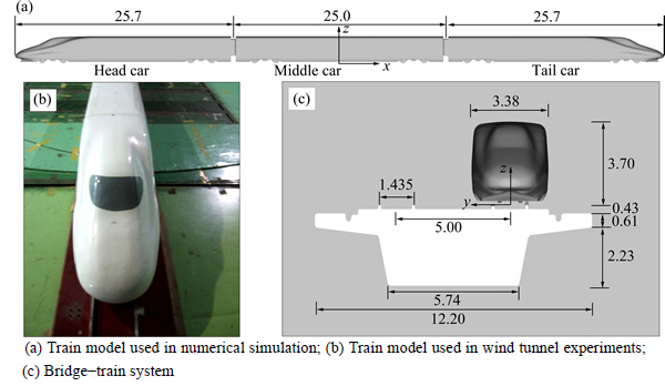
Fig. 1 Geometric models (Unit: m):

To improve the quality of computational grids and accuracy of the solution, some simplifications of the model surface are made. Simplified bogies are retained to simulate the flow near the ground. In addition, the adjacent cars are connected by simplified windshield. Double-line railway bridge (shown in Fig. 1(c)) is a typical type in the application of Chinese high speed railway. In the present work, bridge deck and girder are kept to ensure the main outline, while ventilate and other ancillary facilities are removed. Also, track bed and rails are simulated. The vehicle has a full-scale height of 3.7 m, width of 3.38 m and the length of 76.4 m, whilst the length of head car, middle car, tail car is 25.7 m, 25 m, 25.7 m, respectively. The nominal lateral distance between the contact points of a wheel-set is 1.435 m. The full-scale size of the bridge is shown in Fig. 1(c). The origin of the coordinate system used in this paper is located mid the track on top of rails, and mid the middle car, shown in Figs. 1(a) and (c).

3 Computational domain and boundary conditions

The wind relative to a train U_R is the resultant of a natural wind vector U_w and the wind U_T induced by car running, as shown in (Fig. 2). To investigate velocity distribution near the train, eight vertical lines are marked in Fig. 2(a), in which the black dots represent locations of the lines.

As a running high speed train barely suffers big yaw angle (β) conditions except for the processes of accelerating and decelerating. The relative wind velocity U_R=60 m/s is given to investigate flow around the train on the bridge at 20° yaw angle. Three cases are carried out, train on the windward track on the bridge (WWC), train on the leeward track on the bridge (LWC) and train on the flat ground (FGC).The computation domain used in the present work for WWC is depicted in Fig. 3.

To simulate in a limited zone, the inlet and outlet are required to be far from objective of study to reduce the influences of the upstream and the wake flow. The domain is composed of two inlet boundaries, one located in the front of the vehicle and one on the side, where the latter is used to introduce the cross wind in the domain. The inlet is 10H upstream of the train and the outlet section is 20H from the tail of the train, where H stands for the height of the train. To insure the domain boundaries do not interfere with the flow around the vehicle in a physically incorrect way, the CEN [27] states that the upstream domain shall extend at least eight characteristic heights upstream, and the outlet of the computatinal domain shall be at least 16H downstream of the model. So the length of the domain is enough in this work. The outlets are installed as zero pressure outlets. The surface of bridge deck is about 3H from the ground and 11H from the top. The roof of the domain is set as symmetry. Other walls are set as non-slip wall conditions. The corresponding Reynolds number, Re, is 1.9×10⁶, with the viscosity of air and the H as reference length. The turbulence intensity is chosen to be 5%, corresponding to a turbulent external aerodynamic simulation.

The non-dimensional aerodynamic side force coefficients C_S, lift force coefficient C_L and moment coefficient C_M are defined as

 (1)

where ρ is the air density (1.225 kg/m³); A denotes the nominal vehicle side area, defined as the product L×H (where L is the length of the middle car and H is the height of the car, as indicated in Section 2); F_s is the side force; FL is the lift force; M is the rolling moment (based on the track centreline) [28].

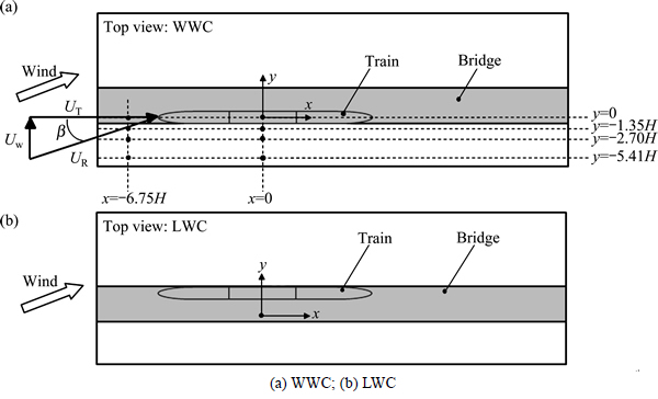
Fig. 2 Definition of windward and leeward cases:

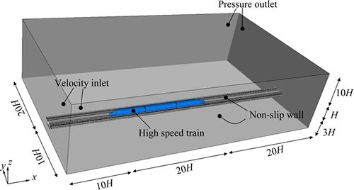
Fig. 3 Computational domain and boundary conditions

4 Numerical method

DES was proposed by SPALART et al [29]. In the early stages of the development of CFD, even massively separated flows had been simulated using RANS methods. Applications of DES predict the flow around a cylinder at high Reynolds number show that the complex flow field are obtained, which can not be obtained by RANS [15, 30]. DES also has been successfully used to study flow of trains, the results compare well to experimental work [16, 21-23]. In the DES approach, the unsteady RANS models are employed in the boundary layer, while the LES treatment is applied to the separated regions. The LES region is normally associated with the core turbulent region where large unsteady turbulence scales play a dominant role. In this region, the DES models recover LES-like subgrid models. In the near-wall region, the respective RANS models are recovered. The resolution of attached boundary layers requires relatively lower grids density. So, DES is not as computationally expensive as LES, that needs a very fine mesh near the wall [31]. The Realizable k-ε based DES model implemented in the commercial CFD solver Fluent is used in this work because of its effectiveness in transporting turbulence quantities [32]. The DES model is similar to the realizable k-ε model, with the exception of the dissipation term in the k equation. The Realizable k-ε RANS dissipation term is modified as

                                   (2)

where △=max(△x, △y, △z), where △x, △y, △z are local cell dimensions in the coordinate directions as shown in Fig. 3. A constant value of 0.61 has been used for the C_DES. The subgrid scale (SGS) model for LES region is Smagorinsky model [33].

5 Computational mesh

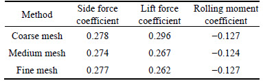
The whole domain was discretized as hexahedral grids using snappy Hex Mesh which is a utility within Open FOAM. The surface grids of train and bridge as well as a cut-plane of the mesh are shown in Fig. 4. Mesh sensitivity was tested using three meshes: coarse mesh, medium mesh, and fine mesh, which consist of 15×10⁶, 30×10⁶, and 50×10⁶ cells, respectively. In order to resolve the boundary layer around the train and the bridge, the max thickness of the first layer is 0.88 mm. The value of y+ over the majority of surface of the train and the bridge is between 30 and 100, which ensures the accuracy computation of wall function. To properly resolve the flow around the train, an extra-refinement was used around the train and the bridge. Table 1 gives time-averaged force coefficients and moment coefficients of three meshes at 20° yaw angle and the U_R is 60 m/s. The results show little difference between the cases, so it can be determined that the results are not a function of mesh density. The medium mesh was employed in this work.

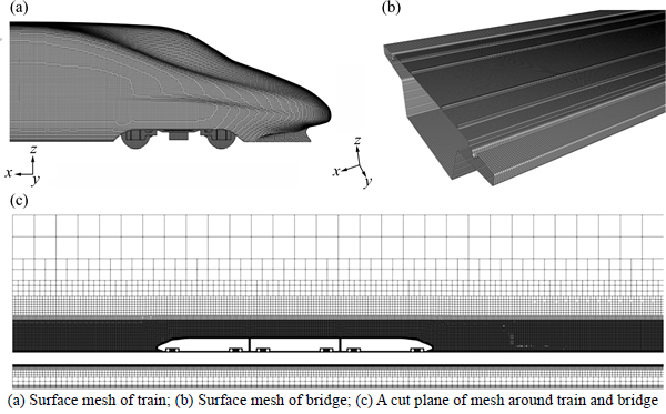
Fig. 4 Computational mesh:

Table 1 Results of head car of three meshes

6 Validation

To ensure the validity of the numerical method, the same method described in Section 4 was used to compute the aerodynamic loads of the same high speed train model on the flat ground at different yaw angles. The yaw angles of five different cases are 0°, 5°, 10°, 15° and 20°, respectively, and the steady relative wind velocity U_R=60 m/s. The computational results are compared with data of wind tunnel experiments. More information about the wind tunnel experiments can be found in Ref. [26], and experimental data in Fig. 5 is obtained from this article. Figure 5 provides the aerodynamic force coefficients of the head car for both the simulations and experiments, which shows that the solution of DES has a good agreement with that of experimental work. Some minor disagreements occur for the lift force coefficient. It is probably due to the difference of the bottom structure between CFD and wind tunnel experiment.

7 Results

7.1 Aerodynamic force

The time steps were set as △t=1.0×10^-4 s, and the total time was 2 s. By averaging the results from 1 s to 2 s, time-averaged aerodynamic force coefficients are obtained. Table 2 gives the time-averaged aerodynamic force coefficients and rolling moment coefficients at 20° yaw angle for the three cases WWC, LWC and FGC. It can be concluded that the aerodynamic side loads of the train on the bridge increase a lot compared to that of the flat ground case, which has been confirmed in the previous literatures [3, 13]. The side fore coefficient C_S of head car for the WWC and LWC cases, compared with the FGC case, increase by 14% and 29%,respectively. Besides, values C_S of middle car for WWC and LWC cases, are 32% and 10% larger than these of FGC case. Furthermore, the C_S of the tail car for WWC case is 45% larger than FGC while 2% smaller than LWC case.

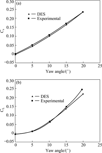
Fig. 5 Comparison between simulation and experiment

Table 2 Side force coefficient C_S and rolling moment coefficient C_M for three cases

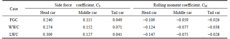
The rolling moment coefficient C_M valuse of the middle car for the WWC and LWC increase by 30% and 27%, respectively. The C_M valuse of the tail car for the WWC and LWC increase by 46% and 1%,respectively. The most notable thing is that the side force and the rolling moment of the head car are greater for the LWC case, while the side force and the rolling moment of the middle car and the tail car are greater for the WWC.

7.2 Velocity distribution

As the flow around train is highly turbulent, the mean velocity is adopted to analyse the wind distribution here. Figure 6 depicts the mean velocity profiles from the numerical simulation at different position in the vertical direction. The velocity magnitude is normalized by the resultant relative wind velocity U_R, and the height is normalized by the vehicle height. Results are presented only for the WWC, since the results of the LWC are analogous. Four vertical lines that are parallel to z axis, at x=-14.6H and x=0, are analysed, Fig. 2(a). The former is located at the halfway between the nose of the head car and the front inlet, and the latter is located at the centre of the train. Due to the friction energy loss in the boundary layer near the floor, the velocity magnitude gradually increases to the same as mainstream velocity magnitude. At x=0, the velocity magnitude rapidly increases near the roof of the vehicle, and the maximum value reaches 1.15, then it gradually decreases to the same as the mainstream velocity magnitude. Comparing the velocity profiles of the four vertical lines, the flow is significantly influenced by the bridge-train system when the air is close to it. As flow separation occurs at the bridge deck edge, the velocity magnitude first decreases then increases at y=-1.35H within a certain height. Along the vertical line, the maximum velocity occurs at z=1.84H for the line x=-14.6H, y=0, and the maximum velocity occurs at z=1.06H for the line x=0, y=0. Comparing the two different location (x=-14.6H and x=0) in the flow field, the maximum velocity increases notablely owing to the increasing of characteristic height of the bridge-train system.

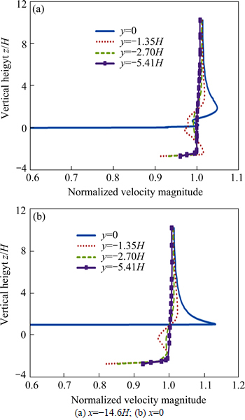
Fig. 6 Mean velocity profiles at different position in vertical direction:

Figure 7 presents results of velocity magnitude at z=1.06H and z=1.84H along two horizontal lines through x=-14.5H and x=0. It can be seen that the speed-up of the flow over the bridge-train system is much greater than that of a single bridge. At the height of z=1.06H, the first peak occurs due to the air separation at the vehicle roof, whilst the second, and the third peaks are a result of the vortex formation at the leeward side. The velocity magnitude gradually recovers to the same as the mainstream. Figure 8 shows the mean normalized velocity magnitude contours of a cut-plane at x=-14.6H. The speed-up effect of the crosswind under the bridge girder is greater than above the bridge deck without the train.

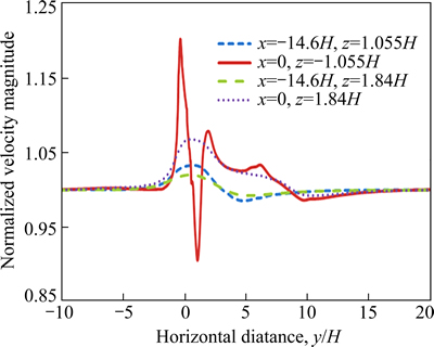
Fig. 7 Mean velocity magnitude profiles at z=1.06H and z=1.84H

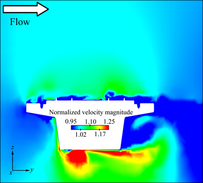
Fig. 8 Velocity contours at x=-14.6H

7.3 Pressure field around trains

Table 2 lists different loads on trains between the three cases (WWC, LWC, FGC). Since aerodynamic force is the result of pressure integration of the train surface, it is necessary to know the pressure distribution around train. Figures 9 and 10 show the contours of train surface mean static pressure coefficient C_p. The pressure coefficient is defined as

                           (3)

where P is the mean static pressure. For the three cases, the pressure on the windward side of train is mostly positive while that of the leeward side is negative. The discrepancy of train’s aerodynamic force is due to the different surface area of positive pressure and negative pressure zone. For the pressure distributions of windward side of the head car are almost the same, the different side forces are mainly due to the distribution of the leeward side, which accounts for larger side force for LWC.

Figure 11 presents the static pressure around the surfaces of the train at 2.44H, 10.34H, 18.24H (Fig. 12) from the nose for the FGC, WWC, and LWC. Although few cross–sections surfaces of the train can not fully account for the loads on it, it can explain some phenomenon to some extent. Among the three positions, the static pressure is quite different at about 135° at x=2.44H, where the violently fluctuation indicates that strong flow separation occurs at the leeward side of the roof. This phenomenon is not apparent at x=10.34H, x=18.24H. Pressure distribution of windward side (0° -45° and 315°-360°) of car body at x=2.44H and x=18.24H are the same for the three cases, which suggests that the different side forces are mainly caused by the different pressure distributions of the leeward side of the car. Pressure of the leeward side of the car on the bridge is smaller than on the flat ground at x=2.44H, leading to larger side loads on the car for the WWC and LWC. The notable difference between the WWC and LWC occurs at the windward side of head car, while pressure distributions on the leeward side of the car are almost the same. And the positive pressure area for the LWC is larger in comparison with the WWC (Fig. 9), resulting in larger side loads on the car. Figure 11(b)shows that the pressure of the windward side of the car is smaller for the LWC than for the WWC at x=10.34H, which is due to the velocity attenuation in the process of airflow over the bridge to the train.

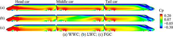
Fig. 9 Pressure distribution of windward side surface of train:

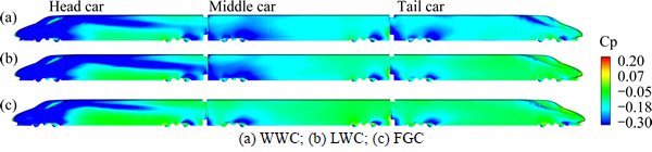
Fig. 10 Pressure distribution of leeward side surface of train:

The cut-planes at 2.44H, 4.24H, 10.34H, 16.44H, 18.24H from the nose of the head car, are shown in Fig. 12. Figure 13 illustrates the flow fields for the WWC case in terms of the mean static pressure coefficient C_p.

A negative pressure area is observed at the vehicle roof, the negative pressure area gradually develops to the leeward side of the train along the longitudinal direction. Figure 13 shows that an obvious vortex generates at the leeward side, and then shedding from the roof. The windward side of the train is under positive pressure, the value gradually decreases along the longitudinal direction. There are several large negative pressure zones at the bottom of the bridge, causing some small vortices near the bottom surface. A small vortex is detected above the gutterway at the windward side, further shown in Fig. 14.

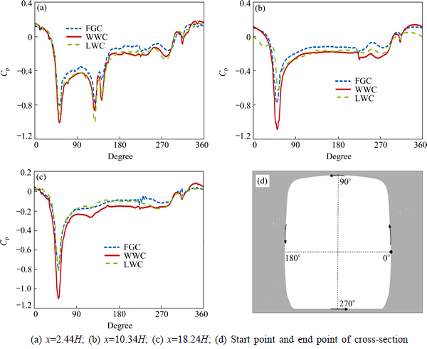
Fig. 11 Static pressure on train cross-section surface:

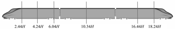
Fig.12 Cut-planes from nose

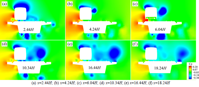
Fig.13 Static pressure coefficient contours on cut-planes at different positions (WWC):

7.4 Flow around trains

As the pressure distribution is caused by the airflow, the flow streamlines around the train need to be researched. The calculated flow fields in cut-planes at 2.44H, 4.24H, 10.34H, 16.44H, 18.24H from the nose of the head car, Fig. 12, are illustrated in Fig. 14 in terms of mean velocity streamlines.

An obvious vortex Vcr1 can be found in the Fig. 14, which generates at around x=2.44H at the leeward side of the roof and develops steadily along the train. The vortex core is gradually away from the car body, and vortex size grows larger then disappears in the wake. A small vortex is detected above the gutterway at the windward side and some various scales of vortices are formed near the bottom surface and leeward side of the girder. As a whole, the incoming flow separates when encountering with the bridge-train system. Part of the flow accelerates over the car or through from bottom of the car, and the rest flow beneath the deck, generating vortices at the corner between the deck and the girder. Another separation occurs at the bottom corner of the girder, and the vortices develop downstream and separate at the leeward corner again, generating much larger vortex at the leeward side of the girder.

Since limited cut-plans can not fully show the flow around the train, the second invariant of the velocity gradient Q is used, Q=0.5×(W×W-S×S), where W is vorticity magnitude, and S is the magnitude of strain rate [28]. To visualize the time-averaged flow, the velocity gradient tensor is replaced by mean velocity gradient tensor. The time-averaged flow around the train using the iso-surface of the second invariant of mean velocity gradient Q is shown in Fig.15.

Figure 15 confirms that the vortex Vcr1 stretches along the leeward side of the train, which is suggested in Fig. 14. In Fig. 15(a), some small structures on train surface are wiped out for better view of the time- averaged flow. The vortex Vcr2 generates at the lower position, and dissipates at the second bogie section of the head car, which can be seen from Fig. 14 at x=6.04H. Several vortices (Vcr3, Vcr4, Vcr5) generate at the leeward side of the roof in the middle car, and develop away from the car, finally mix with Vcr1. This phenomenon also can be seen in the leeward region of the tail car (Fig. 15(d)), however, the vortices do not merge into Vcr1. Another vortex Vcr6 forms at the lower position of the middle car, develops along downstream towards the tail end. In Fig. 14 (at 10.34H, at 16.44H, at 18.24H), this vortex is approximately at a fixed height. In the wake region, vortex Vcr7 generates at the end of the tail car. Some small vortices develop close to the deck floor at the leeward side of the rails, as shown in Fig. 14.

Figure 16(a) shows the iso-surfaces of instantaneous second invariant Q for the WWC. The instantaneous flow structures in the lee-side flow are completely different from that in the time-averaged flow in Fig. 15.

Many compressed structures attach on the windward edge and top of the roofs, and the adhering zones get smaller along the longitudinal direction. The flow has strong unsteady vortex shedding. Many vortices are born on the leeward edge of the roofs. Theses vortices develop downstream, detach and dissipate into the wake region. The eddies develop irregularly, leading to a noticeably turbulent flow at leeward side of train. And the vortices at the leeward side of the tail car are much more than those of the head car, resulting in larger turbulent fluctuation effects on the tail car, as shown in Fig. 17. The instability of the flow at the leeward side disturbs the instantaneous train surface pressure and aerodynamic forces. Figure 17 shows the time histories of the side coefficient and lift coefficient of the train from 1 s to 2 s obtained from the WWC, which indicates the forces fluctuations of the tail car are stronger than that of the head car. Figure 16(b) shows the instantaneous flow structures through the iso-surface of the instantaneous static pressure. The value of the pressure is -450 Pa. The vortices become totally unsteady after the middle car. At the leeward side of the roof of the middle and tail car, the vortices attach to the roof and then detach before another vortex starts to emerge. A coherent structure Vcr1 can be seen in Fig. 16(b), which is similar to the structure in time-averaged flow shown in Fig. 15. And the vortex becomes more unsteady along the longitudinal direction.

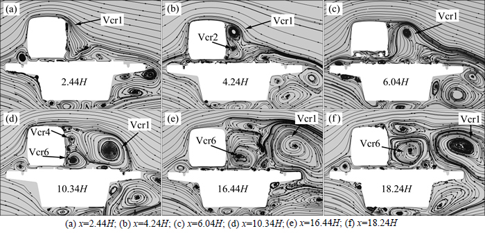
Fig. 14 Mean velocity streamline on cut-planes at different positions (WWC):

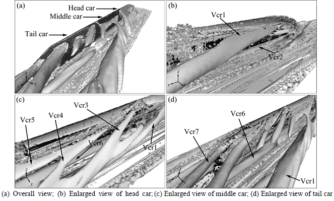
Fig. 15 Iso-surface of time-averaged second invariant of vortices (Q=1000):

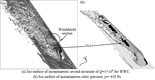
Fig. 16 Instantaneous flow structure around train for WWC:

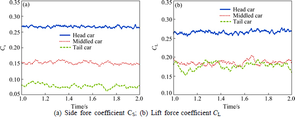
Fig. 17 Time history of the aerodynamic force coefficients from 1 s to 2 s (WWC):

Many vortices with small scales shed from the windshield sections, and merger into the main recirculation region at the leeward side. Figure s 18(a) and (b) show flow structure around train for the LWC, FGC, respectively. Compared with the WWC, the vortices shedding are weaker for both of them, especially in the wake region.

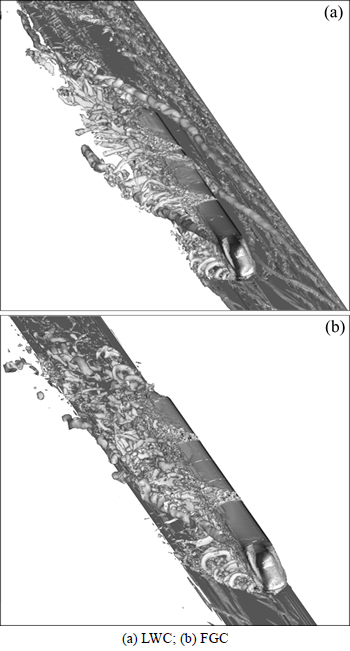
Fig. 18 Iso-surface of instantaneous second invariant of Q=5×10⁴:

8 Conclusions

1) Compared with FGC, the side force coefficients of the head car for the WWC and LWC increase by 14% and 29%, respectively. The side force coefficients of the middle car for the WWC and LWC increase by 32% and 10%, respectively. The side force coefficient of the tail car increases by 45% for the WWC, however, decreases by 2% for the LWC. The most notable thing is that the side force and the rolling moment of the head car are greater for the LWC, while the side force and the rolling moment of the middle car and the tail car are greater for the WWC.

2) Comparing the velocity profiles at different locations, the flow is significantly influenced by the bridge-train system when the air is close to it.

3) For the three cases (WWC, LWC and FGC), the pressure on the windward side of train is mostly positive while that of the leeward side is negative. The discrepancy of train’s aerodynamic force is due to the different surface area of positive pressure and negative pressure zone. For the pressure distributions of windward side of the head car are almost the same, the different side forces are mainly due to the distribution of the leeward side, which accounts for larger side force for LWC.

4) The vortex Vcr1 stretches along the leeward side of the train. The vortex Vcr2 generates at the lower position, and dissipates at the second bogie section of the head car. Several vortices (Vcr3, Vcr4, Vcr5) generate at the leeward side of the roof in the middle car, and develop away from the car, finally mix with Vcr1. This phenomenon also can be seen in the leeward region of the tail car, however, the vortices do not merge into Vcr1. Another vortex Vcr6 forms at the lower position of the middle car, develops along downstream towards the tail end, and the vortex is approximately at a fixed height. In the wake region. A vortex Vcr7 generates at the end of the tail car. Some small vortices develop close to the deck floor at the leeward side of the rails.

5) Many vortices are born on the leeward edge of the roofs. Theses vortices develop downstream, detach and dissipate into the wake region. The eddies develop irregularly, leading to a noticeably turbulent flow at leeward side of train. In addition, many vortices with small scales shed from the windshield sections, and merger into the main recirculation region at the leeward side.

References

[1] HEMIDA H, KRAJNOVIC S. LES study of the influence of the nose shape and yaw angles on flow structures around trains [J]. Journal of Wind Engineering and Industrial Aerodynamics, 2010, 98(1): 34-46.

[2] BAKER C J. The simulation of unsteady aerodynamic cross wind forces on trains [J]. Journal of Wind Engineering and Industrial Aerodynamics, 2010, 98(2): 88-99.

[3] SUZUKI M, TANEMOTO K, MAEDA T. Aerodynamic characteristics of train/vehicles under cross winds [J]. Journal of Wind Engineering and Industrial Aerodynamics, 2003, 91(1/2): 209-218.

[4] TIAN Hong-qi. Research progress in railway safety under strong wind condition in China [J]. Journal of Central South University: Science and Technology, 2010, 41(6): 2435-2443. (in Chinese)

[5] GUO W W, XIA H, de ROECK G, LIU K. Integral model for train-track-bridge interaction on the Sesia viaduct: Dynamic simulation and critical assessment [J]. Computers & Structures, 2012, 112: 205-216.

[6] TIAN Hong-qi. Aerodynamics of high speed train [M]. Beijing: China Railway Publishing House, 2007: 214-265. (in Chinese)

[7] DORIGATTI F, STERLING M, BAKER C J, QUINN A D. Crosswind effects on the stability of a model passenger train-A comparison of static and moving experiments [J]. Journal of Wind Engineering and Industrial Aerodynamics, 2015, 138: 36-51.

[8] BOCCIOLONE M, CHELI F, CORRADI R, MUGGIASCA S. Crosswind action on rail vehicles: Wind tunnel experimental analyses [J]. Journal of Wind Engineering and Industrial Aerodynamics, 2008, 96(5): 584- 610.

[9] BAKER C J, JONES J, LOPEZ-CALLEJA F, MUNDAY J. Measurements of the cross wind forces on trains [J]. Journal of Wind Engineering and Industrial Aerodynamics, 2004, 92(7/8): 547-563.

[10] DIEDRICHS B, SIMA M, ORELLANO A, ZIMMERMANN C. Crosswind stability of a high-speed train on a high embankment [J]. Proceedings of the Institution of Mechanical Engineers Part F-Journal of Rail and Rapid Transit, 2007, 221(2): 205-225.

[11] CHELI F, RIPAMONTI F, ROCCHI D, TOMSINI G. Aerodynamic behaviour investigation of the new EMUV250 train to cross wind [J]. Journal of Wind Engineering and Industrial Aerodynamics, 2010, 98(4): 189-201.

[12] DORIGATTI F, STERLING M, ROCCHI D, BELLOLI M, QUINN A D. Wind tunnel measurements of crosswind loads on high sided vehicles over long span bridges [J]. Journal of Wind Engineering and Industrial Aerodynamics, 2012, 107: 214-224.

[13] YANG Ming-zhi, YUAN Xian-xu, LU Zhai-jun, HUANG An-jie. Experimental study on aerodynamic characteristics of train running on Qinghai-Tibet railway under cross winds [J]. Journal of Experiments in Fluid Mechanics, 2008, 22(1): 76-79. (in Chinese)

[14] HEMIDA H, KRAJNOVIC S, DAVIDSON L. Large eddy simulations of the flow around a simplified high speed train under the influence of cross-wind [C]// Proc 17th AIAA Computational Dynamics Conference. Toronto, Ontario, Canada: AIAA, 2005: 5354.

[15] SQUIRES K D, KRISHNAN V, FORSYTHE J R. Prediction of the flow over a circular cylinder at high Reynolds number using detached-eddy simulation [J]. Journal of Wind Engineering and Industrial Aerodynamics, 2008, 96(10): 1528-1536.

[16] FLYNN D, HEMIDA H, SOPER D, BAKER C J. Detached-eddy simulation of the slipstream of an operational freight train [J]. Journal of Wind Engineering and Industrial Aerodynamics, 2014, 132: 1-12.

[17] HEMIDA H, BAKER C. Large-eddy simulation of the flow around a freight wagon subjected to a crosswind [J]. Computers & Fluids, 2010, 39(10): 1944-1956.

[18] CHELI F, RIPAMONTI F, ROCCHI D, TOMASINI G. Aerodynamic behaviour investigation of the new EMUV250 train to cross wind [J]. Journal of Wind Engineering and Industrial Aerodynamics, 2010, 98(4): 189-201.

[19] BETTLE J, HOLLOWAY A G L, VENART J E S. A computational study of the aerodynamic forces acting on a tractor-trailer vehicle on a bridge in cross-wind [J]. Journal of Wind Engineering and Industrial Aerodynamics, 2003, 91(5): 573-592.

[20] SESMA I, SANCHEZ G, VINOLAS J, RIVAS A, AVILASANC- HEZ S. A 2D computational parametric analysis of the sheltering effect of fences on a railway vehicle standing on a bridge under crosswinds [J]. Proceedings of the Institution of Mechanical Engineers, Part F: Journal of Rail and Rapid Transit, 2013: 0954409713504395.

[21] S, GEORGII J, HEMIDA H. DES of the flow around a high-speed train under the influence of wind gusts [C]// 7th International ERCOFTAC Symposium on Engineering Turbulence Modeling and Measurements, Limassol, Cyprus: IEEE, 2007. DOI: 10.11091/THETA.2007.363410

[22] DIEDRICHS B. Aerodynamic crosswind stability of a regional train model [J]. Proceedings of the Institution of Mechanical Engineers, Part F: Journal of Rail and Rapid Transit, 2010, 224(6): 580-591.

[23] FAVRE T, DIEDRICHS B, EFRAIMSSON G. Detached-eddy simulations applied to unsteady crosswind aerodynamics of ground vehicles [M]. Progress in Hybrid RANS-LES Modelling. Berlin, Heidelberg: Springer, 2010: 167-177.

[24] COOPER R K. The effect of cross-winds on trains [J]. Journal of Fluids Engineering, 1981, 103(1): 170-178.

[25] KHIER W, BREUER M, DURST F. Flow structure around trains under side wind conditions: A numerical study [J]. Computers & Fluids, 2000, 29(2): 179-195.

[26] ZHANG Zai-zhong, ZHOU Dan. Wind tunnel experiment on aerodynamic characteristic of streamline head of high speed train with different head shapes [J]. Journal of Central South University Science and Technology, 2013, 44(6): 2063-2068. (in Chinese)

[27] CEN 14067-4. Railway applications-aerodynamics–Part 4: requirements and test procedures for aerodynamics on open track [S].

[28] MIAO Xiu-juan, GAO Guang-jun. Influence of ribs on train aerodynamic performances [J]. Journal of Central South University, 2015, 22: 1986-1993.

[29] SPALART P R, JOU W H, STRELETS M, ALLMARA S R. Comments on the feasibility of LES for wings, and on a hybrid RANS/LES approach [J]. Advances in DNS/LES, 1997, 1: 4-8.

[30] SIMA M, GURR A, ORELLANO A. Validation of CFD for the flow under a train with 1:7 scale wind tunnel measurements [C]// Proceedings of the BBAA VI International Colloquium on Bluff Bodies Aerodynamics and Applications. Milano, Italy, 2008.

[31] SPALART P R, DECK S, SHUR M L, TRAVIN A. A new version of detached-eddy simulation, resistant to ambiguous grid densities [J]. Theoretical and Computational Fluid Dynamics, 2006, 20(3): 181-195.

[32] SHIH T H, LIOU W W, SHABBIR A, YANG Z, ZHU J. A new k-ε eddy viscosity model for high reynolds number turbulent flows [J]. Computers & Fluids, 1995, 24(3): 227-238.

[33] BOU-ZEID E, MENEVEAU C, PARLANGE M. A scale-dependent Lagrangian dynamic model for large eddy simulation of complex turbulent flows [J]. Physics of Fluids, 2005, 17(2): 025105.

(Edited by DENG Lü-xiang)

Foundation item: Project(U1534210) supported by the National Natural Science Foundation of China; Project(14JJ1003) supported by the Natural Science Foundation of Hunan Province, China; Project(2015CX003) supported by the Project of Innovation-driven Plan in Central South University, China; Project(14JC1003) supported by the Natural Science Foundation of Hunan Province, China; Project(2015T002-A) supported by the Technological Research and Development program of China Railways Cooperation

Received date: 2015-10-27; Accepted date: 2016-03-02

Corresponding author: GAO Guang-jun, Professor, PhD; Tel: +86-731-82656673; E-mail: gjgao@csu.edu.cn