J. Cent. South Univ. Technol. (2009) 16: 0458-0466
DOI: 10.1007/s11771-009-0077-4

A novel resource co-allocation model with constraints to
budget and deadline in computational grid
HU Zhi-gang(胡志刚)1, 2, XIAO Peng(肖 鹏)1
(1. School of Information Science and Engineering, Central South University, Changsha 410083, China;
2. School of Software, Central South University, Changsha 410083, China)
Abstract: To address the issue of resource co-allocation with constraints to budget and deadline in grid environments, a novel co-allocation model based on virtual resource agent was proposed. The model optimized resources deployment and price scheme through a three-side co-allocation mechanism, and applied queuing system to model the work of grid resources for providing quantitative deadline guarantees for grid applications. The validity and solutions of the model were presented theoretically. Extensive simulations were conducted to examine the effectiveness and the performance of the model by comparing with other co-allocation policies in terms of deadline violation rate, resource benefit and resource utilization. Experimental results show that compared with the three typical co-allocation policies, the proposed model can reduce the deadline violation rate to about 3.5% for the grid applications with constraints to budget and deadline. Also, the system benefits can be increased by about 30% compared with the those widely-used co-allocation policies.
Key words: co-allocation; computational grid; grid economy; queuing theory; deadline
1 Introduction
Grid computing has emerged as a promising network computing platform that aggregates heterogeneous and distributed resources for solving high-end applications, which frequently require access to multiple resources across virtual organizations [1]. Therefore, resource co-allocation is always the key issue in grid computing, and various co-allocation frameworks have been developed in various grid systems [2-4]. These frameworks mainly focus on co-allocation service architecture and programming interfaces for grid applications. None of them has addressed the issue of resource co-allocation with the constraints to budget and deadline.
As complementary to co-allocation frameworks, many co-allocation policies and models were proposed. LEINBERGER et al [5] proposed two backfilling-based heuristics for K-resource co-allocation. Their studies showed that load-balancing policy outperforms classical policies over 50% in terms of mean response time. MOHAMED and EPEMA [6] proposed a close-to-files policy, which tried to place jobs on clusters closing to the input files so as to reduce communication overhead. HE et al [7] proposed two policies (ORT and OMT) to address co-allocation. ORT aimed to optimize mean response time for non-real-time jobs, while OMR was designed to achieve the optimal mean deadline miss rate for soft real-time job streams. To evaluate the performance of various co-allocation policies, BUCUR and EPEMA [8-9] conducted extensive experiments in large-scale grid system. Based on their experimental results on grid test-bed DAS-2 [10], they made an important conclusion that workload-aware policies were effective to reduce the mean response time and obtain better load-balance. Unfortunately, most of the above policies aimed to improve the system performance metrics, but few of them took the users’ QoS constraints into account.
In order to co-allocate resources for those applications with constraints to budget and deadline, grid economy [11] has been introduced into grid systems, such as Spawn [12], Popcon [13], and Nimrod-G [14]. For instance, Nimrod-G provided three adaptive policies for deadline and budget constrained resources allocation [15]: cost optimization, time optimization, and conservative time optimization. Although economic model has been proven to be an effective method for resource allocation in distributed environments, it has two shortcomings that cannot be ignored: (1) economic models bring about extra communicational and computational overhead to applications [11]; (2) in presence of high-end applications that require co- allocating multiple resources across sites, the price negotiation process is often low-efficient [15].
Recently, game theory has been widely used to resource allocation in grid computing [16-17]. These studies assumed that the participants in co-allocation game were selfish, and then proposed many methods to find the equilibrium solution of resource price scheme. Unlike those studies, KHAN and AHMAD [18] classified game-based co-allocation model into three types: cooperative, semi-cooperative and non- cooperative. By extensive simulations, they indicated that agent-based cooperation model was effective for resource co-allocation. However, KHAN’s cooperative model was of very high computational complexity and did not support co-allocation under deadline constraint, which inspires us to find the more efficient method.
This work focused on co-allocation with constraints to budget and deadline in high-performance computational grid. A class of novel entities, namely virtual resource agents (VRAs), were introduced into conventional co-allocation model. The VRAs organized resources belonging to different sites into virtual sites through a three-side gaming mechanism, and provided an efficient price mechanism to meet applications’ budget constraint and to improve resource benefit.
2 VRA-based co-allocation framework
The VRA-based co-allocation model considered in this work is shown in Fig.1, which is based on the conventional multicluster computational grid [2].
The VRA-based co-allocation model consists of several computing elements (CEs), each representing a homogeneous cluster, a set of VRAs, and a meta- scheduler. In this model, meta-scheduler works as follows: when a job arrives, the meta-scheduler selects suitable VRAs based on the job’s budget and deadline, then dispatches the job to those selected VRAs. The VRAs work as follows: all the VRAs buy resources from the system at a uniform price, and then sell them to the clients at different retail prices. The distinctive difference between VRAs and local scheduler is that VARs can encompass resources across the boundaries of sites. Furthermore, the VRAs can adjust their resource quantities at runtime. The objectives of introducing VRAs to the system are as follows: (1) making a reasonable resource price scheme to meet job’s budget constraint as well as improving resource benefit; (2) modeling the working of resources so as to provide quantitative guarantees for job’s deadline constraint.
In this model there are three types of participants: resource providers, VRAs and clients. The resource providers and VRAs cooperate with each other, as they both aim at maximizing resources utilization and benefits. On the other hand, the relationship between the VRAs and the clients is non-cooperative, as the clients hope to minimize their costs, which would inevitably lower down the benefits of resource providers. According to the above analysis, it can be seen that the three types of participant form a three-side allocation model similar to client-retailer-producer model [19].
3 Analysis of VRA-based co-allocation model
3.1 Utility functions
The utility functions of the three types of participants are defined in this section. In the next sections, analysis and solutions of the model are based on these functions.
As the resource providers sell their resources to VRAs at a uniform price p*, its utility function US is defined as
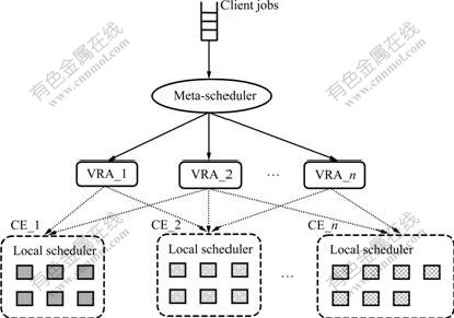
Fig.1 VRA-based co-allocation framework
 p*
p* (1)
(1)
where si is the amount of computing resources in the ith computing element. Uniform price p* is to facilitate the resource providers to calculate their resource benefits. The decision of resource retail price is handled to VRAs. This strategy is similar to producer-retailer-client model [19].
The VRAs are denoted as Vi (i∈[1, …, n]). Let ci (ci>0) represent the resource quantity in Vi, ρi (0<ρi<1) be the resource utilization rate of Vi. Thus, the utility function of Vi is defined as
 (2)
(2)
where pi is the resource retail price set by Vi for clients.
Client job j is characterized by a 3-tuple:j, bj, dj>, where rj is the resource demand, bj is the budget constraint, and dj refers to the deadline constraint. Let J represent the VRAs set that has been allocated to job j, and  be the amount of resources allocated from Vi to
execute job j, then the cost of job j is  . As the
guarantee of deadline constraint is not a quantitative measurement, it is mapped into a probability. Let Ei be the random event representing that Vi (i∈J) can guarantee the deadline constraint of job j, then, the probability of which the deadline of job j can be satisfied
is expressed as  So the utility function of job
j is defined as
 (3)
(3)
3.2 Cooperative model analysis
In the cooperative model, the resource providers aim to find a suitable p* that can maximize resource benefit, and the VRAs need to decide their resource quantities. Therefore, the solution of the cooperative model is a pair *, C>, where C=(c1, c2, …, cn) is a parameter representing the resource quantities in each VRA. For the convenience of representation, some definitions are given as follows.
Definition 1 S+(p*)={Vi| >0, i∈[1, …, n]} is the set of VRAs with positive benefit at p*; S-(p*)= {Vi|<0, i∈[1, …, n]} is the set of VRAs with negative benefit at p*; and S0(p*)={Vi|=0, i∈[1, …, n]} is the set with zero benefit.
Definition 2 At *, ci>, Vi will be in balancing state if Vi∈S0(p*); at *, (c1, …, cn)>, the VRA-based model will be in balancing state if  Vi (i∈[1, …, n]) satisfies Vi∈S0(p*).
Definition 3 The global benefit is the sum of all the resource providers’ benefits and the VRAs’ benefits,
noted as 
Theorem 1 If the VRA-based model is in balancing state at *, (c1, …, cn)>, adjusting *, (c1, …, cn)> will not affect the global benefit UG.
Proof Let  …,
…,  represent the benefits of VRAs at *, (c1, …, cn)>. According to the definition of balancing state, it can be known that
 Vi(i∈[1, …, n]) (4)
So, the global benefit UG at *, (c1, …, cn)> is
 p*
p* (5)
(5)
Let  …,
…,  represent the benefits of VRAs at *+?p*, (c1+?c1, c2+?c2, …, cn+?cn)>, where ?p*∈±R, ?ci∈±Z. Then, the total benefit of all the VRAs is
 (p*+?p*)=
-?p* (6)
(6)
Therefore, the global benefit  at *+?p*, (c1+?c1, c2+?c2, …, cn+?cn)> is

(p*
p* (7)
The total resource quantity is fixed, which means
that Combining Eqn.(5) with Eqn.(7), it can be known that

Theorem 2 If the VRA-based model is not in balancing state at *, (c1, …, cn)>, the global benefit UG can always be increased by adjusting *, (c1, …, cn)>.
Proof As the model is not in balancing state, the global benefit UG at *, (c1, …, cn)> is
 (8)
(8)
So, UG will be independent of p* when the model is not in balancing state. If p* is adjusted to  where
where  pkρk and
  p*, the model will satisfy the following conclusions at *, (c1, …, cn)>.
(1) The model is still not in balancing state (or else it will contradict with the precondition of the theorem).
(2) According Formula (8), the global benefit remains the same as that at *, (c1, …, cn)>.
(3) The VRA Vk is in balance state, that is, Vk∈S0( ).
).
According to Conclusion (1), it can be known that  satisfies Vi∈S+() or Vi∈S-(), where i≠k.
If Vi∈S+(), the resource quantities of Vk and Vi can be adjusted to  and
and  respectively, where ?δ>0. Since Vk∈S0(p*), any adjustment of Vk’s resource quantity will not affect the global benefit. However, as Vi∈S+(), increasing Vi’s resource quantity can increase the global benefit. So, the global benefit at <, (c1, …,
  …,
…,  …, cn)> is larger than that at *, (c1, …, cn)>. If Vi∈S-(), the analysis and conclusion are similar to the above, and the only difference is that ?δ<0.
Lemma 1 Being in balancing state is the sufficient and necessary condition for VRA-based model to obtain the maximal global benefit.
Proof According to Theorem 1, it can be known that the global benefit may be maximal or minimal when the VRA-based model is in balancing state. By the conclusion of Theorem 2, there is always a method to increase the global benefit when the model is not in balancing state. So, the global benefit can only be maximal instead of being minimal when the model is in balancing state, or the method shown in Theorem 2 can be used to increase the global benefit.
Based on the conclusion of Lemma 1, the model can improve the global benefit through repeatedly adjusting *, (c1, …, cn)> to make the model in (or near to) balancing state. In fact, the proof of Theorem 2 shows a method to do that. However, the method shown in Theorem 2 is low-efficient, because there is only one VRA being in balancing state after each adjustment. So, a more efficient approach to adjusting *, (c1, …, cn)> is developed.
Given the model is not in balancing state at *, (c1, …, cn)>, let <  …,
…,  > represent the new solution of the model. Based on the definition of balancing state, if satisfies Eqn.(9), the model is the nearest to balancing state.
F= (9)
(9)
It is clear that the solution of Eqn.(9) is 
 At a new the benefit of each VRA will
be changed correspondingly. Therefore, the resource quantity of VRAs is adjusted as follows: (1) if Vi∈S+(), increase the resource quantity of Vi; (2) if Vi∈S-(), decrease the resource quantity of Vi; (3) if Vi∈S0(), remain the resource quantity of Vi unchanged.
In summary, the process of resolving of the cooperative model is repeatedly adjusted *, (c1, …, cn)>. The adjustment of p* makes the model near to balancing state, and the adjustment of (c1, …, cn) is to deploy more resources to those VRAs that are capable of obtaining more benefits. The algorithm of adjusting *, (c1, …, cn)> is shown as follows. In the algorithm, Steps 3-10 are to categorize VRAs into two sets: one needs to enlarge their resource quantity, the other needs to reduce their resource quantity. In Step 13, two heuristics are used to adjust the resource quantity between VRAs: (1) deploy the resources belonging to the same CEi to the same VRA [6, 20]; and (2) more resources will be deployed to the VRA that can obtain the best benefit. The complexity of the algorithm is O(n), when n is the number of CE in the system. Parameter ?k is the decrement/increment of resource quantity in each adjustment. The analysis of the effects of ?k on model performance can be seen in simulations.
Algorithm of adjusting *, (c1, …, cn)> is as follows.
Input: *, (c1, …, cn)>
Output: < …, >
1. Begin
2. 
3. for i=1 to n
4. calculate  at the new price
5. if Vi∈S+() then
6. add i to expand_list
7. else if Vi∈S-()
8. add i to shrink_list
9. end if
10. end for
11. for each i in shrink_list
12. 
13. find j in expand_list, which satisfies one of the two conditions: (1) the amount of resources comes from CEi in Vi is maximal; (2)  is maximal in the VRAs that needs to be expanded.
14. 
15. end for
16. End
3.3 Non-cooperative model analysis
The meta-scheduler assigns jobs to the VRAs based on client utility function  The clients tend to select the VRAs with lower retail price pi and higher resource quantity ci, because those VRAs are more likely to be able to meet job’s budget and deadline constraints. Although a high value of retail price might lead to better benefits for the VRA, its resource utilization rate will lower down too. On the other side, a low retail price can lead to high resource utilization rate, however, if the benefits of the VRA become negative, its resource quantity will be reduced in the next adjustment of *, (c1, …, cn)>. So, the solutions of the no-cooperative model between VRAs and client jobs are the resource retail prices (p1, …, pn).
According to the VRA model, if the resource utilization rate is in high level, a VRA can reduce its retail price, yet still maintain its benefit in a relative high level. So the retail price is a decreasing function of resource utilization rate, which is denoted as pi(ρi). Then, the utility function of Vi can be rewritten as follows:
 (10)
(10)
Let  Eqn.(11) can be obtained. Denote the solution of Eqn.(11) as
  It is clear that the maximal value of can be obtained when
  So
So  is called as the optimal resource utilization rate of Vi.
 (11)
(11)
However, Vi cannot set its ρi as by itself. Instead, it can only change its retail price to influence the clients’ resource selection so as to optimize its benefit. By comparing the difference between and ρi, a VRA can decide whether increasing or decreasing its retail price. The process is as follows: if ρi<, Vi will decrease its price to  else Vi will increase its price to
  This process will be performed repeatedly until an optimal retail price scheme is achieved. Parameter ?p is the decrement/ increment of resource retail price. The effect of ?p on model performance will be analyzed in simulations.
Finally, the probability that the deadline constraint of a job can be guaranteed should be figured out. It is assumed that the arrival of jobs in Vi is a Poisson process with rate λi, and the execution time of jobs follows exponential distribution with rate μi. Therefore, a VRA can be modeled as a M/M/ci queuing system [21]. So, the resource utilization rate of Vi can be expressed as ρi=λi/(ciμi).
Let ψi be a random variable representing the number of waiting jobs in Vi. According to queuing theory [21], the probability that there are k waiting jobs in Vi is
 (12)
(12)
where
 (13)
(13)
Let ωi be a random variable representing the completion time (including waiting time and execution time) of a job in Vi, then the probability that Vi can guarantee the job’s deadline dj is expressed as
Pr{Ei}=Pr{ωi≤dj} (14)
For M/M/ci queuing system, the service rate is ciμi, which means that the system can complete ciμi jobs in a unit time. So, the amount of jobs that Vi can complete in period dj is ciμidj. Therefore, the probability that Vi can guarantee a job whose deadline dj is equal to the probability that the waiting jobs in Vi are not more than ciμidj-1. By Eqns.(12)-(14), it can be known that
Pr{Ei}=Pr(ωi≤dj)=Pr{ψi≤ciμi(dj-1)}=
 (15)
(15)
Therefore, Formula (3) can be rewritten into Eqn.(16), which is used by meta-scheduler to select the best VRAs to execute client jobs.
 (16)
(16)
4 Experiments and performance evaluation
4.1 Experimental setting
The simulations are conducted by using GridSim [22], a distributed resource management and a scheduling simulator, to evaluate the performance of the VRA-based co-allocation model. A multicluster computational grid model is constructed, which consists of 10 clusters. The detail settings of each cluster are listed in Table 1.
In simulations, the basic workload (jobs stream) is
Table 1 Settings of grid model in simulations

generated by using Lublin-Feitelson model [23], which is derived from the workload logs of real supercomputers. It consists of 10 000 jobs, and each is characterized by its arrival time, resource demands, and estimation of execution time. The resource demands of each job are enlarged by f times, where f is uniformly distributed in [10.0, 20.0], so as to simulate the co-allocation in large- scale grid environments. As the basic workload does not include deadline, each job is appended with a deadline constraint as
dj=tj+ ?k (17)
where dj is the deadline, tj is the arrival time, is the execution time, and k is a random variable that is uniformly distributed in [1.5, 5.5].
4.2 Performance comparison
Firstly, the performance of four co-allocation
policies is compared in terms of deadline violation rate, resource benefit, and resource utilization rate. The four policies are round robin policy (RR_P) [24], capability- based random policy (CR_P) [25], cluster minimized policy (CM_P) [20], and virtual resource agent policy (VRA_P). The fourth policy (VRA_P) is proposed in this paper, in which the meta-scheduler dispatches a job to suitable VRAs based on job’s utility function shown in Eqn.(16).
The experimental results of the four policies are listed in Table 2. The details of each CE’s benefit are shown in Fig.2. Deadline violation occurs if the system cannot actually meet a job’s deadline constraint. To analyze the effects of resource utilization rate on resource benefit, the resource utilization rates of the four policies at runtime are shown in Fig.3, and the average utilization rates of CEs shown listed in Fig.4.
As shown in Table 2, although RR_P is of the highest resource utilization rate, its deadline violation rate is also the highest, which leads to its resource benefit in a very low level. This is because RR_P dispatches jobs to clusters in turn, which can quickly full-utilize resources in a balancing fashion. However, RR_P does not take deadline constraint into account, so many jobs cannot be completed in their deadline constraints. As to CR_P, it is a static-performance-driven co-allocation policy. As shown in Fig.4, most of the jobs are scheduled on a few of high-performance clusters (i.e. CE_2, CE_4 and CE_9) when CR_P is used. Such load-imbalance results in that CR_P’s resource utilization rate is the lowest (only 12%). Even so, as CR_P takes into account the resources’ static capacity while co-allocating resources, its deadline violation rate (13%) is about a half of the RR_P’s, which makes its resource benefit more than RR_P’s (about 20%).
Table 2 Violation rates and benefits of four co-allocation policies
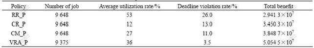
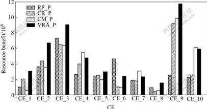
Fig.2 Detail benefits of CEs
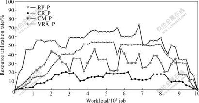
Fig.3 Resource utilization rates at runtime
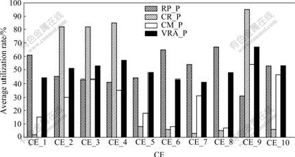
Fig.4 Average utilization rates of CEs
From Fig.3, it can be seen that CM_P outperforms VRA_P in terms of resource utilization rate for the first 2 000 jobs. After that, the resource utilization rate of the VRA_P gradually surpasses that of CM_P, and does not fluctuate so dramatically as that of CM_P does. The reason is that: VRA_P co-allocates resources based on jobs’ utility function, so a few powerful resource that can better guarantee jobs’ deadline and budget constraints have been frequently selected, which makes VRA_P suffer from load-imbalance of the beginning of simulation just like CR_P. However, VRA_P is capable of adjusting its retail prices and VRAs’ resource quantities for optimizing the benefits of both the system and clients. This feedback mechanism helps VRA_P find an efficient solution to resources’ deployments and prices. After the first 2 000 jobs, the retail prices and resource quantities of all the VRAs have been adjusted to a suitable level. As shown in Fig.2, the average benefits of each CE are in proportion to their computing power when VRA_P is used. As VRA_P selects the resources with an optimal probability to meet a job’s deadline constraint, its violation rate is only 3.5%, which is significant lower than that of the other three policies. Such lower violation rate makes its resource benefit the highest compared with that of the other three policies. Therefore, it can be concluded that VRA_P can provide reliable QoS guarantees for applications in terms of budget and deadline.
4.3 Effects of ?k and ?p on model performance
In VRA_P, ?k and ?p are the decrement/increment of resource quantity and retail price, respectively. Extensive simulations are conducted to examine the effects of these two parameters on VRA_P in terms of deadline violation rate and resource benefit. The results are shown in Fig.5 and Fig.6, respectively. Also, the performance of scheduling is shown in Fig.7.
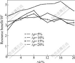
Fig.5 Effects of ?k and ?p on resource benefits
The simulation tests are carried out at four different values of ?p (5%, 10%, 15% and 20%) combining with gradually increasing ?k from 0 to 20%. As shown in Fig.5 and Fig.6, the violation rate and resource benefit are the most optimal when ?k=16% and ?p=10%. When ?p>10%, the resource benefit becomes irregular with the increase of ?k. This is because large ?p means that the
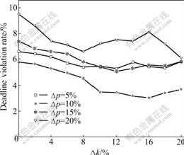
Fig.6 Effects of ?k and ?p on deadline violation rate
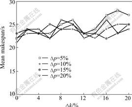
Fig.7 Effects of ?k and ?p on mean makespan
retail price fluctuates dramatically, as VRA_P tends to select those VRAs with low retail prices. So it is hard for the VRAs to obtain the optimal retail price for maximizing the resource benefit. When ?p=50%, VRAs have to take a long time to get the optimal retail price, so the resource benefit cannot be as much as that when ?p=10%. According to the analysis in Section 3.2, we know that it is difficult for the VRA-based model to reach balancing state when large value of ?p is used. On the other side, small value of ?p makes the speed of convergence to balancing state too slow. In Fig.7, the performance of scheduling is measured by the mean makespan. It is clear that the makespan fluctuates slightly when ?k<14%. Only when ?k>14% the effects of ?p become apparent, but the difference of makespan for different ?p is always less than 7%. So, it can be concluded that the effects of ?p and ?k on scheduling are very small.
5 Conclusions
(1) Although the proposed VRA_P co-allocation does not perform better than CR_P and CM_P in terms of average resource utilization rate, its deadline violation rate (about 3.5%) is much better than that of the two co-allocation policies, which shows that VRA-based co-allocation model is of practical value for those applications with deadline constraint, such as real-time grid jobs.
(2) According to the statistic of runtime resource utilization rate and individual CE’s utilization rate, the feedback mechanism in VRA_P helps the resource providers find an efficient solution for resource providers to optimize their resource benefits.
(3) By extensive simulations, the performance of the VRA_P is investigated by using different combinations of ?k and ?p. The optimal values of ?k and ?p in these simulations are ?k =16% and ?p=10%. It is noteworthy that such results are obtained in the special grid model setting. So, different grid systems should set ?k and ?p according to the systems’ characteristics, such as jobs’ features, quantity and performance of resources. So, adaptive mechanism to find the optimal values of ?k and ?p is the next research direction of this work.
References
[1] Foster I, Kesselman C. The grid: Blueprint for a new computing infrastructure [M]. Singapore: Elsevier Inc, 2004.
[2] Czajkowski K, Foster I, Kesselman C. Resource co- allocation in computational grids [C]// Proceedings of Inter Symp on High Performance Distributed Computing. California: IEEE Computer Society Press, 1999: 219-228.
[3] Lewis M J, Ferrari A J, Humphrey M A. Support for extensibility and site autonomy in the legion grid system object model [J]. Journal of Parallel and Distributed Computing, 2003, 63(5): 525-538.
[4] Wolski R, Brevik J, Obertelli G, Spring N. Writing programs that run EveryWare on the computational grid [J]. IEEE Trans on Parallel and Distributed Systems, 2001, 12(10): 1066-1080.
[5] Leinberger W, Karypis G, Kumar V. Job scheduling in the presence of multiple resource requirements [C]// Proceedings of ACM/IEEE Conf on Supercomputing. Portland: IEEE Computer Society Press, 1999.
[6] Mohamed H H, Epema D H J. An evaluation of the close-to-files processor and data co-allocation policy in multiclusters [C]// Proceedings of Inter Conf on Cluster Computing. San Diego: IEEE Computer Society Press, 2004: 287-298.
[7] HE L G, Jarvis S A, Spooner D P. Allocating non-real-time and soft real-time jobs in multiclusters [J]. IEEE Trans on Parallel and Distributed Systems, 2006, 17(2): 99-112.
[8] Bucur A I D, Epema D H J. Scheduling policies for processor co-allocation in multicluster system [J]. IEEE Trans on Parallel and Distributed Systems, 2007, 18(7): 958-962.
[9] Bucur A I D, Epema D H J. The performance of processor co-allocation in multicluster systems [C]// Proceedings of IEEE/ACM Inter Symp on Cluster Computing and the Grid. Tokyo: IEEE Computer Society Press, 2003: 302-309.
[10] Bal H, Bhoedjang R R, Hofman R. The distributed ASCI supercomputer project [J]. ACM Operating Systems Review, 2000, 34(4): 76-96.
[11] Buyya R, Abramson D, Venugopal S. The grid economy [J]. Proceeding of the IEEE, 2005, 93(3): 698-714.
[12] Waldspurger C A, Hogg T, Huberman B A, et al. Spawn: A distributed computational economy [J]. IEEE Trans on Software Engineering, 1992, 18(2): 103-117.
[13] Nisan N, London S, Regev O. Globally distributed computation over the internet: The POPCORN project [C]// Proceedings of Inter Conf on Distributed Computing Systems, Amsterdam: IEEE Computer Society Press, 1998: 592-601.
[14] Abramson D, Giddy J, Foster I. High performance parametric modeling with nimrod/G: killer application for the global grid? [C]// Proceedings of Inter Symp on Parallel and Distributed Processing. Chicago: IEEE Computer Society Press, 2000.
[15] Buyya R. Economic-based distributed resource management and scheduling for grid computing [D]. Melbourne: Monash University, 2002.
[16] Kwok Y K, Hwang K, Song S. Selfish grids: Game-theoretic modeling and NAS/PSA benchmark evaluation [J]. IEEE Trans on Parallel and Distributed Systems, 2007, 18(5): 621-636.
[17] Rzadca K, Trystram D, Wierzbicki A. Fair game-theoretic resource management in dedicated grids [C]// Proceedings of Inter Symp on Cluster Computing and the Grid. Rio de Janeiro: IEEE Computer Society Press, 2007: 343-350.
[18] Khan S U, Ahmad I. Non-cooperative, semi-cooperative, and cooperative games-based grid resource allocation [C]// Proceedings of Inter Symp on Parallel and Distributed Processing. Rhodes Island: IEEE Computer Society Press, 2006.
[19] Osborne M, Rubinstein A. A course in game theory [M]. Cambridge: Massachusetts Institution of Technology Press, 1994.
[20] Mohamed H H, Epema D H J. Experiences with the KOALA co-allocating scheduler in multiclusters [C]// Proceedings of Inter Symp on Cluster Computing and the Grid. Cardiff: IEEE Computer Society Press, 2005: 784-791.
[21] Gross D, Harris C M. Fundamentals of queuing theory [M]. 3rd ed. New Jersey: John Wiley and Sons Inc, 1998.
[22] Buyya R, Murshed M. GridSim: A toolkit for the modeling and simulation of distributed resource management and scheduling for grid computing [J]. Concurrency and Computation: Practice and Experience, 2002, 14: 1175-1220.
[23] Lublin U, Feitelson D G. The workload on parallel supercomputers: Modeling the characteristics of rigid jobs [J]. Journal of Parallel and Distributed Computing, 2003, 63(11): 1105-1122.
[24] Dumitrescu C L, Raicu I, Foster I. The design, usage, and performance of GRUBER: A grid usage service level agreement based brokering infrastructure [J]. Journal of Grid Computing, 2007, 5(1): 99-126.
[25] Berten V, Goossens J, Jeannot E. On the distribution of sequential jobs in random brokering for heterogeneous computational grids [J]. IEEE Trans on Parallel and Distributed Systems, 2006, 17(2): 113-124.
(Edited by CHEN Wei-ping)
Foundation item: Project(60673165) supported by the National Natural Science Foundation of China
Received date: 2008-08-22; Accepted date: 2008-10-27
Corresponding author: HU Zhi-gang, Professor; Tel: +86-731-8836300; E-mail: zghu@mail.csu.edu.cn

