Trans. Nonferrous Met. Soc. China 23(2013) 2736-2742

Direct pre-stack depth migration on rugged topography

Zhu-sheng ZHOU, Gao-xiang CHEN

School of Geosciences and Info-Physics, Central South University, Changsha 410083, China

Received 1 December 2012; accepted 22 April 2013

Abstract: Engineering seismic exploration aims at shallow imaging which is confused by statics if the surface is uneven. Direct pre-stack depth migration (DPDM) is based on accurate elevations of sources and receivers, by which static correction is completely abandoned before migration and surely the imaging quality is remarkably improved. To obtain some artificial shot gathers, high-order staggered-grid finite-difference (FD) method is adapted to model acoustic wave propagation. Since the shot gathers are always disturbed by regular interferences, the statics still must be applied to supporting the interference elimination by apparent velocity filtering method. Then all the shot gathers should be removed back to their original positions by reverse statics. Finally, they are migrated by pre-stack reverse-time depth migration and imaged. The numerical experiments show that the DPDM can ideally avoid the mistakes caused by statics and increase imaging precision.

Key words: undulating topography; seismic modeling; static correction; apparent velocity filtering; direct pre-stack depth migration

1 Introduction

The classic seismic exploration theory is based on the assumption, which is almost impossible in practice, of horizontal surface and homogeneous medium. To meet the demands of the rapidly developing economy, it is necessary to carry out seismic prospecting in mountainous areas where the conventional seismic method is always thought to be unsuitable [1-3]. Though the static correction can help to improve the exploration effect, it is still unable to clear up the so-called residual static correction introduced by different emergency angles and it will lead to incomplete correction and waveform distortion. This problem emerges extremely seriously in engineering seismic exploration [4], since its detecting depth is much lower than that of the oil and gas exploration. After the normal static correction, there came some modified versions, such as refraction static correction, tomographic static correction and time- shifting static correction. Despite the improvement, the residual static correction has not yet been eliminated thoroughly.

Furthermore, the readability and signal to noise ratio of the entire seismogram will be badly disturbed by the disordered wave fields reflected from the complex surface and subsurface. Besides, uneven earth’s surface always means variable lateral velocities, which can be another factor that keeps the static correction from be using in processing. And the conventional post-stack migration is also unable to yield an accurate image of underground layers, since it requires horizontally unchanged velocity and flat surface. Fortunately, the newly developed method, pre-stack migration, just features in mapping complicated geologic frameworks even under the rugged surface condition. There are two general categories composing the pre-stack migration: one is pre-stack time migration and the other is the popular pre-stack depth migration (PDM) which will be used in this work. The PDM was first used in the 1970s, and at the very beginning it was just a theoretical method because of the high computational cost. However, the computer technology has made such a rapid progress in the past decades that the implementation of the PDM in practice has become a reality.

There are alternatives of the PDM. The Kirchhoff integration method (KIM) is the famous one of them, which is widely applied to industries due to the relatively simple and fast computational realization [5]. But this solution is just a high frequency approximation of the wave equation, and it is incapable of tackling the multi-path and blind-area problems which is inevitable if complex geological model is involved [6]. The other choices are always the wave equation based solutions, including time-space, frequency-space and frequency- wave number domain methods. All of them are better in imaging complicated subsurface structures than the KIM, and obviously the computation cost is no longer a limitation to their application with the help of the sophisticated hardware and software. It is worth to mention that the full-wave equation based reverse-time migration (RTM) avoids the separation of up-going wave and down-going wave which makes it possible to image the turning and prismatic waves, and the usual dipping angle limitation in migration is also decreased [7,8]. During the whole process of the RTM, all the wave values of each time step of each grid point are so completely used that the final image contains adequate kinematic information as well as dynamic information.

In this work a new procedure, in which the static correction will be entirely excluded before migrating, is suggested to the RTM for engineering seismic exploration in the situation of undulating surface. Roughly, this new solution consists of six primary steps, namely, source wave field simulation, first-break static correction, linear interference suppression, reverse first-break static correction, reverse-time wave field simulation and imaging. Here we can find that before the shot gather is migrated, all the influence caused by the static correction will be removed thanks to the step four.

2 Experimental

2.1 Source wavefield simulation

To obtain the solution of the full-wave equation the core step is either the source wave field simulation or the reverse-time data extrapolation. The FD method is an ideal option for solving wave equation due to its advantages of efficient execution and low requirement on computer. In this work, the popular high-order staggered- grid FD method [9,10] is selected to perform modeling and reverse-time wave extrapolation based on the first-order speed-stress acoustic equation. And the PML boundary condition [11,12] is applied to absorbing the reflection generated by model truncation. The first-order differential equation that the PML is considered to work efficiently is given by

                (1)

where u_x and u_z, v_x and v_z denote pressure and speed of each material point in both the horizontal and vertical directions; v_p and ρ are the velocity and the density, respectively; d¹(x) and d²(z) work as absorbing coefficients of the PML. Substituting the second-order accuracy time difference term and the 2Nth-order accuracy space difference term, given by expressions (2), into expression (1) simply, we get the discrete version which is suitable for computing on a PC.

    (2)

where are the 2Nth-order difference operator coefficients [13] determined by the following equation:

,

n=1, 2, …, N

To test the finite-difference schemes and the PML boundary condition, a 1000 m×1000 m homogeneous geological model (named Model 1) with a constant velocity of 3000 m/s is assumed. The spatial grid interval is 5 m both horizontally and vertically and the time increment is 0.5 ms so as to ensure stability and suppress grid dispersion. The Ricker wavelet with a dominant frequency of 50 Hz is introduced as the explosive source.

Figure 1(a) shows a wave field snapshot, taken at time 0.2125 s with the source located at the geometric center of the model, which displays intense boundary reflections. While in Fig. 1(b) the reflections are remarkably eliminated by the PML layers matched around the computational area. The comparison of Figs. 1(a) and (b) demonstrates that the finite-difference schemes used here are stable and the PML boundary does work well. Actually, it can be estimated by dividing the maximum reflected amplitude by that of the direct wave that the reflectivity in this case is reduced to 0.065%. Besides, the usual numerical dispersion can also be ignored here since it is too small to be considerable compared to the dominant signals in Fig. 1.

2.2 Reverse-time wave extrapolation

Reverse-time wave extrapolation is another pivotal procedure of the PDM since no successful migration will be achieved without accurate reverse-time wave field. The governing equations are the same as those of the forward ones except for the opposite signs of the absorbing coefficients d¹(x) and d²(z) in Eq. (1).

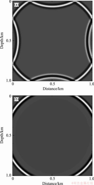
Fig. 1 Snapshot taken at 0.2125 s without PML (a) and with PML (b)

Figure 2(a) shows four snapshots at different times produced form Model 1. Figure 2(b) shows a single-shot gather, in which the PML boundaries are applied, obtained from the model surface. Figure 2(c) presents the four rebuilt reverse-time wave fields according to Fig. 2(b). Comparing the triangular area in Fig. 2(c) to that in Fig. 2(a), the upgoing wave fields are correctly rebuilt by the reverse-time difference schemes. It is worth to say that, in Fig. 2(c) some fuzzy wave fields appear symmetrically on the left and right side of the model. These are the unexpected turbulences caused by the abrupt discontinuities of the phase axis in Fig. 2(b). Fortunately, they can be suppressed by applying the cross-correlation imaging condition at each time step of the imaging procedure.

2.3 Imaging condition

Better imaging condition helps to optimize the final migrated seismogram, especially in complicated cases, and it will affect the computational efficiency as well. In this section, three different imaging conditions based on the Claerbout-created cross-correlation method are discussed. The first one is the traditional type which directly cross-correlates the source wave-field with the reverse-time wave field according to Eq. (3) under the basic assumption that the source wave field stands only for down-going wave field and the receiver for up-going. Unfortunately, in many cases this assumption is invalid, particularly when some challenging geological environments and uneven surfaces are involved. To improve the quality of migrated images, we can divide the cross-correlated image either by the source illumination (Eq. (4)) or the receiver illumination (Eq. (5)) respectively [14-17].

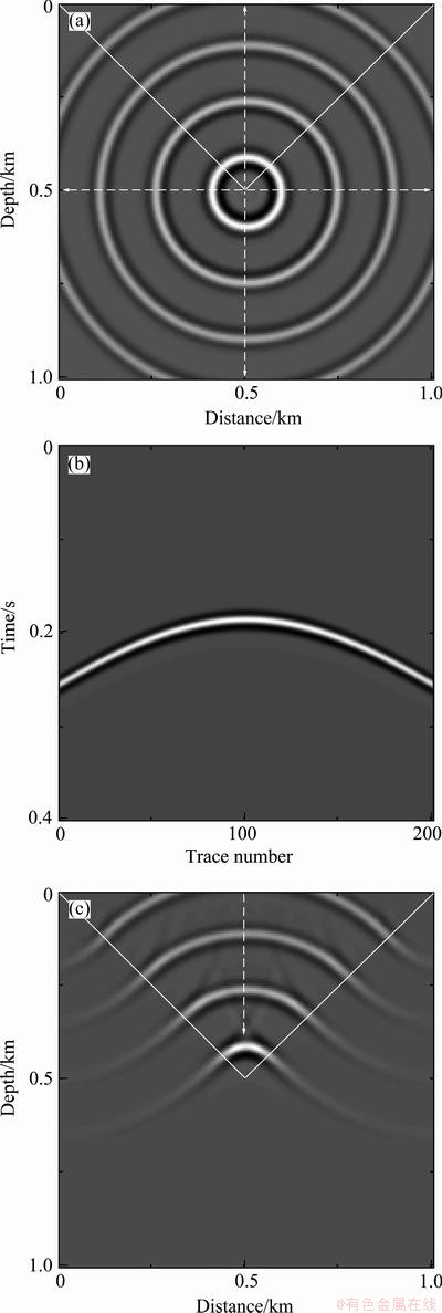
Fig. 2 Forward wavefields (a), single-shot gather produced from surface of Mode l (b), and result (c) of reverse-time wave fields according to Fig. 2(b)

                (3)

                (4)

                (5)

where I(z, x) denotes the final migrated image; S_i(t, z, x) is the down-going wave field at time t in the ith shot gather; R_i(t, z, x) is the up-going wave field; N, T, z and x stand for shot number, total recording time, vertical and horizontal coordinates, respectively.

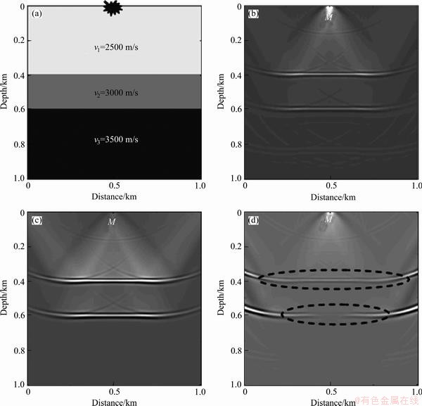
Fig. 3 Model 1 (a) and reproduced stratum structures under cross-correlation imaging condition (b), source illumination imaging condition (c), receiver illumination imaging condition (d)

Figure 3(a) presents a three-layered level geological model with the constant density of 2.0 g/cm³. Here the wave equation is approached by the second-order temporal and ten-order spatial FD with 5 m grid interval in both x and z directions and the time increment is 0.5 ms. A single-shot gather is produced, which has not been displayed in Fig. 3, by 201 geophones placed on the surface of the model with interval of 5 m, and the source locates at point M (x=500, z=0). Figures 3(b)-(d) show the migrated images under three different imaging conditions based on the single-shot gather. Figure 3(b) is yielded by Eq. (3). It is obvious that the whole section is suppressed by the strong low frequency artifact (called illumination effect usually) between the first layer and the source. This phenomenon will become more serious as the impedance contrasts increases. Normalizing the cross-correlation with SI results in Fig. 3(c) where the strong artifacts near the source are massively diminished and the shallow reflectors are strengthened. While Fig. 3(d), generated from the normalization of the cross-correlation with RI, shows contrast situation compared to Fig. 3(c) that the far away reflectors are strengthened while the shallow ones are decreased (the areas trapped by the two ellipses in Fig. 3(d)). However, both the second and the third imaging conditions are better than the first one if the model is much more complicate.

3 Results and discussion

The main purpose of this work is discussing the direct pre-stack depth migration method under the circumstance of undulating topography. All the work done before this section is the precondition that ensures the achievement of the DPDM. In this section, three distinguished undulating surface models are assumed to test the effect of the DPDM. The model parameters and structures are shown in Figs. 4, 5 and 6, and all the three share the same grid spacing and FD parameters. Both the depth and horizontal distance are dispersed every 5 m and the accuracy of FD is second-order time and tenth-order space. The boundary reflections are absorbed by the PML.

Figure 4(a) shows a relatively simple model and Fig. 4(b) results from the DPDM using cross-correlation corresponding to Fig. 4(a). In this case, both the shape and the depths of the reflectors are migrated correctly. The model in Fig. 5(a) is a little more complicated than the former one because of the three different uneven reflectors. Fortunately, the DPDM is still capable of recovering the structures shown in Fig. 5(b) by cross- correlation condition. Figure 6(a) shows a fault model composed of several discontinuous uneven reflectors and Fig. 6(b) shows the migrated image by the DPDM. Because of the challenging geological structures, the receiver illumination imaging condition should be applied to imaging the interfaces instead of the cross-correlation condition so as to highlight the deep structures. What need to be pointed out is the less information near the boundaries than the center of the model, that causes the intermittent path axis illustrated by the ellipse in Fig. 6(b), but it has nothing to do with the DPDM algorithm itself. Comparing the amplitudes of the different reflectors in Fig. 4(b)-Fig. 6(b) respectively, one can find that the DPDM is able to reveal the correct dynamic information because the amplitude distributions are equivalent to the reflection coefficients shown in Fig. 4(a)-Fig. 6(a). All the three models are processed according to the sequence mentioned at the end of the Introduction, in which the static correction is totally avoided before migration, which is the key point of the DPDM.

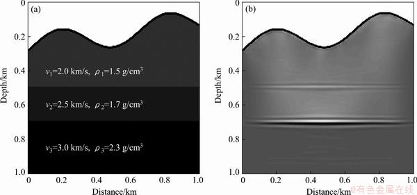
Fig. 4 Undulating surface model 2 (a) and migrated result (b) by DPDM (using cross-correlation)

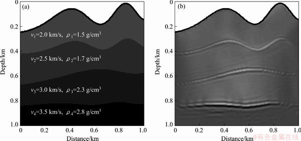
Fig. 5 Undulating surface model 3 (a) and migrated result (b) by DPDM (using cross-correlation)

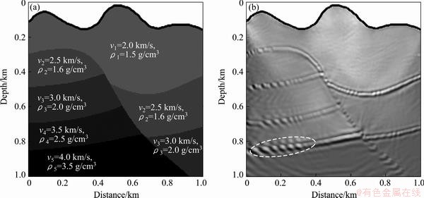
Fig. 6 Undulating surface model 4 (a) and migrated result (b) by DPDM (using receiver illumination condition)

4 Conclusions

1) It can be concluded that the DPDM is capable of achieving accurate structure characteristics and perfect dynamic information under the situation of undulating topography. A great progress has been made in the quality of the seismogram migrated by the DPDM compared to the conventional process due to the avoidance of static correlation and dynamic correlation.

2) The full wave equation DPDM is suitable for any migration aperture and dipping angle thanks to the low approximation of the partial differential wave equation and the full use of the forward and reverse-time wave fields. In addition, it can be applied to the case of lateral variation of velocity.

3) The source illumination or the receiver illumination imaging condition is suitable for mapping complex structures and large impedance contrasts. Besides, it is worth to mention that the source illumination condition pays more attention to the shallow reflectors while the receiver illumination condition for deep ones.

References

[1] LEI Xiu-li, LI Zhen-chun, KONG Xue, LV Hong-qian. Prestack depth migration using complex Pade approximations for irregular surface [J]. Progress in Geophys, 2012, 27(5): 2100-2106. (in Chinese)

[2] ZHANG Hao, ZHANG Jian-feng. 3D prestack time migration including surface topography [J]. Chinese Journal of Geophys, 2012, 55(4): 1335-1344. (in Chinese)

[3] TANG Wen, WANG Shang-xu, WANG Zhi-ru. Perfectly matched layer absorbing boundary condition of finite element prestack reverse time migration in rugged topography [J]. Procedia Engineering, 2012, 37(6): 304-308.

[4] HAO Jun, YANG Rui-juan, WU Jing, XUE Lei. Processing of static correction problems of seismic data in the complex surface [J]. Complex Hydrocarbon Reservoirs, 2011, 4(3): 34-37.

[5] WANG Yang-guang, KUANG Bin. Prestack reverse-time depth migration on rugged topography and parallel computation realization [J]. Oil Geophysical Prospecting, 2012, 47(2): 266-271.

[6] MCMECHAN G A, CHEN H W. Implicit static corrections in pre-stack migration of common-source data [J]. Geophysics, 1990, 55(6): 756-760.

[7] LIU Fa-qi, ZHANG Guan-quan. An optimized wave equation for seismic modeling and reverse time migration [J]. Geophysics, 2009, 74(6): 153-158.

[8] WILLIAM W, SYMES. Reverse time migration with optimal check pointing [J]. Geophysics, 2007, 72(5): 215-221.

[9] DU Qi-zhen, LIN Bin. Numerical odeling of seismic wavefields in transversely isotropic media with a compact staggered-grid finite-difference scheme [J]. Applide Geophysics, 2009, 6(1): 42-49.

[10] DONG Liang-guo, MA Zai-Tian. A staggered-grid high-order difference method of one-order elastic wave equation [J]. Chinese Journal of Geophysics, 2000, 4(3): 411-419. (in Chinese)

[11] WANG Yong-gang, XING Wen-jun. Study of absorbing boundary condition by perfectly matched layer [J]. Journal of China University of Petroleum, 2007, 31(1): 19-24. (in Chinese)

[12] XU Yi, ZHANG Jian-feng. An irregular-grid perfectly matched layer absorbing boundary for seismic wave modeling [J]. Chinese Journal of Geophysics, 2008, 51(5): 1521-1526. (in Chinese)

[13] YANG Liu, MRINAL K S. An implicit staggered-grid finite-difference method for seismic modeling [J]. Geophys, 2009, 179: 459-474.

[14] CHATTOPADHYAY S, MCMECHAN G A. Imaging condition for pre-stack reverse-time migration [J]. Geophysics, 2008, 73(3): 81-89.

[15] HIDEVRAND S T. Rverse-time migration:Impedance imaging condition [J]. Geophysics, 1987, 52(8): 1060-1064.

[16] SAVA P, FOMEL S. Time-shift imaging condition in seismic migration [J]. Geophysics, 2006, 71(6): 209-217.

[17] LOEWENTHAL D, LIANG Ze-hui. Two methods for computing the imaging condition for common-shot pre-stack migration [J]. Geophysics, 1991, 56(3): 378-381.

地形起伏条件下的直接叠前深度偏移

周竹生，陈高祥

中南大学 地球科学与信息物理学院，长沙 410083

摘  要：工程地震主要解决浅中层地质问题，然而在复杂地表条件下静校正会严重影响浅中部地层的成像精度。基于起伏地形条件下的直接叠前偏移，通过研究适用于精确炮检点高程的新的成像条件，完全避开了静校正处理，从而提高成像质量。首先从正演出发，利用高阶交错网格有限差分法精确模拟地表起伏条件下的纵波波场，并得到复杂地表条件下的单炮记录。再将炮检点通过静校正方法进行野外一次静校正，以便于利用视速度滤波法除去规则干扰。然后，再进行反静校正处理，把各道数据又重新恢复到野外实际高程点，最后直接利用带地形的单炮记录进行叠前深度偏移。模型结果表明，直接叠前偏移处理能够很好地避免静校正带来的误差，大幅度地提高浅中部地层的成像精度。

关键词：起伏地形；波场模拟；静校正；视速度滤波；直接叠前深度偏移

(Edited by Hua YANG)

Corresponding author: Gao-xiang CHEN; Tel: +86-15258879287; E-mail: hncschengaoxiang@126.com

DOI: 10.1016/S1003-6326(13)62791-0