J. Cent. South Univ. (2016) 23: 1690-1699

DOI: 10.1007/s11771-016-3223-9

Multi-physics analysis of permanent magnet tubular linear motors under severe volumetric and thermal constraints

LI Fang(李方)^{1, 2}, YE Pei-qing(叶佩青)^{1, 2, 3}, ZHANG Hui(张辉)^{1, 2}

1. Department of Mechanical Engineering, Tsinghua University, Beijing 100084, China;

2. Beijing Key Lab of Precision/Ultra-precision Manufacturing Equipments and Control (Tsinghua University),

Beijing 100084, China;

3. State Key Laboratory of Tribology (Tsinghua University), Beijing 100084, China

Central South University Press and Springer-Verlag Berlin Heidelberg 2016

Abstract: Permanent magnet tubular linear motors (TLMs) arranged in multiple rows and multiple columns used for a radiotherapy machine were studied. Due to severe volumetric and thermal constraints, the TLMs were at high risk of overheating. To predict the performance of the TLMs accurately, a multi-physics analysis approach was proposed. Specifically, it considered the coupling effects amongst the electromagnetic and the thermal models of the TLMs, as well as the fluid model of the surrounding air. To reduce computation cost, both the electromagnetic and the thermal models were based on lumped-parameter methods. Only a minimum set of numerical computation (computational fluid dynamics, CFD) was performed to model the complex fluid behavior. With the proposed approach, both steady state and transient state temperature distributions, thermal rating and permissible load can be predicted. The validity of this approach is verified through the experiment.

Key words: tubular linear motor; multi-physics; coupling; lumped-parameter; temperature prediction

1 Introduction

Linear motors have served in a wide range of industrial fields where high speed and high acceleration are required. According to their shapes, linear motors can be classified into three types: flat, U-shaped and tubular ones. In general, tubular linear motors (TLMs) are more prominent for high force density [1-2] because the axially symmetric configuration improves utilization of magnetic energy. Therefore, for applications under severe environments (limited installation space, poor cooling condition, etc.), TLMs are a better option to some extent. A brief review on the modeling of linear motors (especially TLMs) is given below.

During the design stage of a linear motor, the electromagnetic modeling aims to predict its some basic parameters, such as thrust force, back electromotive force, and copper loss, while the thermal modeling aims to predict the temperature distribution and assess the thermal rating. The modeling of the two physical fields can be realized via either analytical methods (semi-analytical method based on Maxwell’s equations, lumped-parameter method, etc.) [3-8] or numerical methods (finite element method, etc.) [9-10]. It is noteworthy that the two physical fields are not independent of each other. Multi-physics or coupling analysis enables data exchange between them in one-direction or bi-direction to ensure high computation accuracy [11-13]. For one-direction coupling, these physical models are solved in successive steps. The results of the first analysis act as the inputs of the second analysis. For example, the iron loss from the magnetic model is imported into the thermal model to predict the temperature distribution [14]. For bi-direction coupling, these physical fields are solved simultaneously with all the necessary variables taken into account. For example, in the electromagnetic computation the electric resistivity is updated according to the precedent thermal computation; in the thermal computation, the temperature rise is predicted with Joule loss obtained from the electromagnetic computation [15-16].

This work deals with a set of parallel permanent magnet TLMs (N'M) arranged in N rows and M columns, as shown in Fig. 1. This special device is used for a radiotherapy machine. Each TLM drives one leaf independently so as to form an arbitrary radiation field (as shown in the bottom in Fig. 1). A detailed description of radiotherapy machines is presented in Ref. [17]. Due to limited installation space, the gap between two adjacent TLMs is much smaller than the diameter of the TLMs. Although cooling air driven by external fans is used to take heat away to the ambient, the TLMs are still at high risk of overheating. Therefore, it is crucial to predict the performance of the TLMs such as temperature distribution, thermal rating and permissible load. To guarantee good prediction accuracy, the fluid model of the surrounding air should be considered in addition to the electromagnetic and the thermal models of the TLMs. Thus, a multi-physics analysis approach is proposed in this work considering the coupling effects of the three physical fields. In view of large computation cost of finite element methods, a combined analytical-numerical approach is put forward. Both the electromagnetic and the thermal models are based on lumped-parameter methods, whereas the fluid modeling is via computation fluid dynamics (CFD).

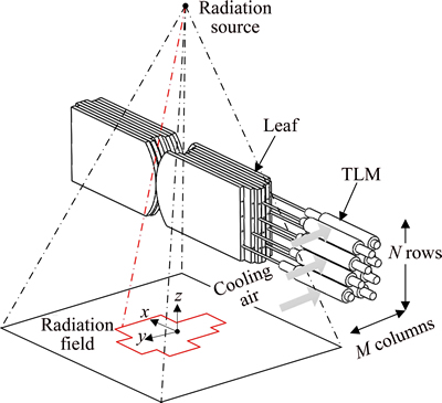
Fig. 1 Schematic diagram of TLMs used for radiotherapy machine

2 Structure of TLMs

The structure of the TLMs is shown in Fig. 2. The fixed part (stator) consists of a polymer tube, windings and a back iron from the inside out. The windings contain two phases arranged alternately. The function of the polymer tube is to support and fasten the windings. The moving part (translator) is composed of axially magnetized permanent magnets and iron pieces. The translator is surrounded by a non-magnetic stainless steel sleeve, the thickness of which can be neglected compared with the other dimensions. The ‘moving translator’ installation is selected for the advantage of less moving mass and space-fixed cables. The main parameters of the TLMs are given in Table 1.

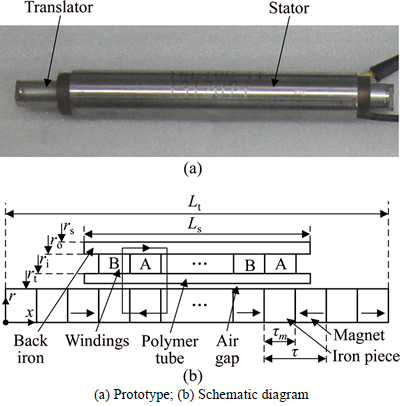
Fig. 2 Structure of TLMs:

Table 1 Main parameters of TLMs

3 Electromagnetic, thermal and fluid modeling

3.1 Electromagnetic modeling

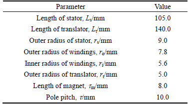
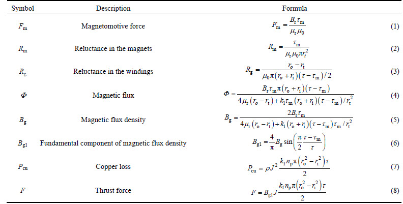
Due to the axial symmetry of the TLMs, a 2-D lumped-parameter magnetic circuit is established as shown in Fig. 3(b). Only one of n_p poles is considered, where n_p represents the total number of the poles. The magnetic circuit is analogous to an electric circuit: magnetomotive force to electromotive force, reluctance to resistance and magnetic flux to current. Several assumptions are made: 1) the flux density distribution along x direction is a square wave; 2) the magnetic drop in the iron is neglected; 3) the armature reaction is neglected. The parameters of the magnetic circuit are given in Table 2 [5-6], where B_r and m_r are the remanence and the relative recoil permeability of the permanent magnets respectively, m₀=4p'10^-7 H/m, r is the electric resistivity of the copper, k_f is defined as the filling factor, i.e. the ratio of the copper volume to the total volume, and k_l is introduced to estimate the leakage flux.

For an application with a wide temperature range, the influence of the temperature rise on the remanence of the permanent magnets should be considered. Their relationship is modeled as

                    (9)

where a_pm and T_pm are the temperature coefficient and the mean temperature of the permanent magnets respectively, and B_r0 is measured at T₀ (20 °C). The sintered NdFeB (Grade N52) is selected with a remanence of 1.4 T and a maximum operating temperature of 80 °C.

Fig. 3 Multi-physics analysis approach:

Table 2 Parameters of magnetic circuit

The electric resistivity is also temperature dependent as follows:

                     (10)

where a_cu and T_cu denote the temperature coefficient and the mean temperature of the copper respectively, and r₀ is measured at T₀.

Substituting Eqs. (5)-(7) into Eq. (8) and combining Eqs. (9) and (10), the thrust force F can be rewritten as

                (11)

It clearly shows the dependence of the thrust force on the temperature rise of the permanent magnets and the copper.

3.2 Thermal modeling

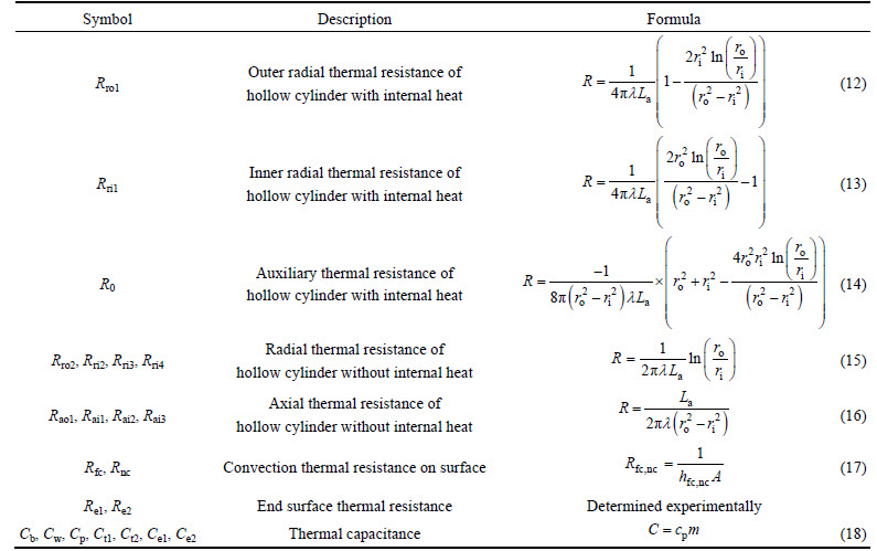
The lumped-parameter thermal network of the TLMs is also similar to an electric circuit: temperature to voltage, power to current, thermal resistance to electric resistance and thermal capacitance to electric capacitance [18]. To establish a thermal network, the TLMs should be divided into several segments connected through nodes.Each segment is represented by a thermal resistance. From Fig. 2(b), the geometry of the TLMs can be viewed as a combination of a solid cylinder (i.e. translator) and a series of hollow cylinders (i.e. air gap, polymer tube, windings and back iron) from the inside out. Hence, by integrating the thermal models of some basic geometric shapes, the thermal network of the TLMs can be established, as shown in Fig. 3(c). It is also a 2D model due to the axial symmetry. The parameters of the thermal network are given in Table 3 [7-8], where l is the thermal conductivity of the material, r_o and r_i denote the outer and inner radii respectively, L_a is the axial length, c_p is the specific heat, m is the mass of the material, T_tc, T_ts and T_ss represent the temperatures of the translator center, the translator surface and the stator surface respectively, T_cu is the mean temperature of the copper, and T_pm is the mean temperature of the permanent magnets.

The copper loss P_cu is injected into the network at the mean temperature node of the windings. The iron loss and the mechanical loss are both neglected as they only account for a small fraction of the total power loss when the alternating frequency of the magnetic field is not very high and the friction is small. Note that from Table 3 all the thermal resistances can be calculated out based on the material thermal properties and the geometric dimensions, except the convection thermal resistance R_nc on the translator surface and R_fc on the stator surface. They rely on the corresponding convection coefficients h_nc and h_fc , respectively.

Table 3 Parameters of thermal network

The convection coefficient h_nc is associated with the natural convection on the translator surface that is not surrounded by the stator. The empirical correlations for a horizontal cylinder [19] are adopted to estimate h_nc. The Nusselt number Nu depends on the Rayleigh number Ra and the Prandtl number Pr as follows:

             (19)

Then h_nc can be calculated by

                               (20)

and R_nc is

                  (21)

where the outer surface and the end surface of the translator are both included in calculating the contact area. The convection coefficient (h_fc) associated with the airflow on the stator surface will be studied in the next section.

3.3 Fluid modeling

The airflow on the stator surface is similar to that of a tube bank heat exchanger. Numerous empirical correlations derived from either experimental or numerical approaches are available currently for tube bank heat exchangers [20]. However, they are not applicable because the fluid region here is more complex. A CFD software ANSYS CFX is used to solve this problem. CFD is a useful tool to predict the impact of fluid flow on electrical machines [18]. This software is used to determine the convection coefficient (h_fc) on the stator surface.

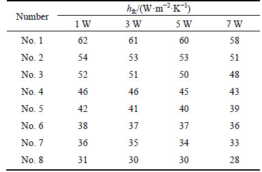
In the CFD simulation, a 3D fluid model is established as the computation domain, as shown in Fig. 3(a). For simplicity, only a single row is modeled (i.e. M=8, N=1), and a hollow tube without interior structure is modeled to represent a TLM. The standard k-ε turbulent model is adopted. The pressure difference between the inlet and the outlet is set to 240 Pa to simulate two external fans, and the inlet temperature is fixed to T₀=20 °C. At the inner surface of each hollow tube, the heat flux density boundary is defined. Its value is equal to the heat dissipation power from the stator surface, i.e. P_fc. A series of simulations are conducted with P_fc ranging from 1 W to 7 W every 2 W. The solution of the CFD simulation when P_fc=5 W is shown in Fig. 3(a). It can be observed that the fluid temperature increases with the increase of the distance from the inlet. The 8 hollow tubes in a row have different convection boundary conditions. By dividing the heat flux density by the corresponding temperature difference, the convection coefficient h_fc is calculated by

              (22)

where N denotes the N-th hollow tube in a row. Table 4 lists the calculated convection coefficient h_fc as a function of the heat dissipation power P_fc of the 8 TLMs in a row. Then the corresponding thermal resistance R_fc is calculated by

                (23)

Table 4 Convection coefficient h_fc (P_fc, N) as function of heat dissipation power P_fc of 8 TLMs in a row

4 Multi-physics analysis

The schematic diagram in Fig. 3 clearly shows the coupling effects of the three physical fields. The copper loss used in the thermal model is determined by the electromagnetic model (linkage A), the latter relys on the temperature information from the former to update the electric resistivity of the copper and the remanence of the permanent (linkages B and C). The input power of the fluid model comes from the thermal model (linkage D), while the convection boundaries of the latter depend on the former (linkage E). On this basis, both the steady state and transient state temperature distributions can be predicted.

4.1 Steady state analysis

In the steady state analysis, the thrust force must be constant and the thermal capacitances are neglected. Based on Kirchhoff laws, each node temperature in Fig. 3(c) has a linear relationship with the copper loss, and the following matrix can be derived:

                    (24)

where R_eq1, R_eq2, R_eq3, R_eq4 and R_eq5 are the corresponding equivalent resistances. Since all the thermal resistances have been calculated up to now, the equivalent resistances can be obtained by simplifying the thermal network. The thermal resistance R_fc is regarded as constant in the steady state analysis.

Substitute T_pm and T_cu in Eq. (24) into Eq. (11), which yields:

       (25)

It is found that there is a one-to-one correspondence between the thrust force and the copper loss. Then replacing P_cu in Eq. (25) by T_tc according to Eq. (24) obtains

       (26)

Figure 4(a) displays the relation between the translator center temperature T_tc and the thrust force F based on Eq.(26). The results of the 8 TLMs in a row as well as a single TLM under the natural convection (h= 8 W/(m²·K)) are all presented. Note that the 8 TLMs in a row have different thermal resistance R_fc values according to Table 4. So they have different relation curves. Analogously, the relationship between the other node temperatures (T_cu, T_ss and T_ts) and the thrust force F can also be obtained easily based on Eqs. (24) and (25), as plotted in Figs. 4(b)-(d). Thanks to the proposed analytical equations, the calculation takes little time. From Fig. 4, the steady state temperature distribution of each TLM in a row under a constant thrust force can be obtained.

4.2 Transient state analysis

In the transient state analysis, the thrust force may vary with respect to time and the thermal capacitances cannot be neglected. So, Eqs. (24)-(26) are not applicable here. An iterative computation process is put forward to predict the transient state temperature distribution, as shown in Fig.5. The input is the trust force F and the output is all the node temperatures (T_cu, T_ss, T_tc, T_pm, and T_ts). In each iterative step Dt, the three steps follow one another: 1) the copper loss P_cu is calculated based on the equation in Fig.5(a) where the temperatures T_pm and T_cu are from the precedent cycle; 2) the heat dissipation power P_fc from the stator surface is calculated, and then the thermal resistance R_fc is obtained based on the relation curve between R_fc and P_fc in Fig. 5(c); 3) all the node temperatures (T_cu, T_ss, T_tc, T_pm and T_ts) are calculated based on the equation in Fig. 5(b) with the obtained copper loss P_cu and thermal resistance R_fc. The relation curve between R_fc and P_fc in Fig. 5(c) is fitted by a quadratic polynomial curve based on Table 4. Using the above iterative computation process, the transient state temperature distribution of each TLM in a row under a time-varying thrust force can be obtained. When the thrust force is constant, the transient state temperature distribution will converge to the steady state one.

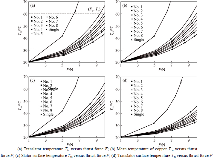
Fig. 4 Steady state analysis:

4.3 Thermal rating and permissible load

From Table 4, it is known that the 8th TLM in a row near the outlet is under the worst cooling condition. So, the overheating of the 8th TLM is most likely to occur. Only the performance of the 8th TLM is analyzed below. As each node temperature increases exponentially with the thrust force, an improper selection of the thrust force may result in a considerable increase in temperature and hence lead to excessive thermal deformation and material failure. To avoid the risk of overheating, it is necessary to take the following limiting factors into consideration comprehensively: 1) The winding temperature should remain below the designated insulation class limit; 2) The irreversible demagnetization of the permanent magnets is not allowed to occur; 3) The thermal deformation of the polymer tube should be kept within a reasonable range. Through contrastive analysis, the irreversible demagnetization of the permanent magnets is most likely to occur with the temperature rise. Therefore, the translator center temperature T_tc should stay below 80 °C, noting that T_tc is the highest temperature of the permanent magnets. In the actual application, T_tc is restricted to 60°C (T_p) for safety and the corresponding thrust force F_p is 9.4 N, as indicated in Fig. 4(a). Therefore, the permissible load should be restricted to F_p.

5 Experimental results

The experiment is carried out on the prototype as shown in Fig. 6(a). The prototype includes 64 TLMs arranged in 8 rows and 8 columns (i.e. M=8, N=8). Two external fans are mounted on two opposite sides to provide forced air cooling. A row of TLMs are tested. The stator surface temperature T_ss is measured through a platinum-based resistance temperature sensor (PT100). As it is not convenient to mount a temperature sensor on the moving translator, the translator surface temperature T_ts is monitored through a thermal imaging infrared camera (NEC H2640). A piece of black tape is stuck onto each translator end to improve the measurement accuracy. Note that from Fig. 4 T_ss T_tc, and T_cu for the same TLM are very close because the radial thermal resistances are much smaller compared with the axial ones due to the slender structure. Therefore, T_ss can be used to estimate T_tc and T_cu such that no extra sensors are needed to place inside the TLMs.

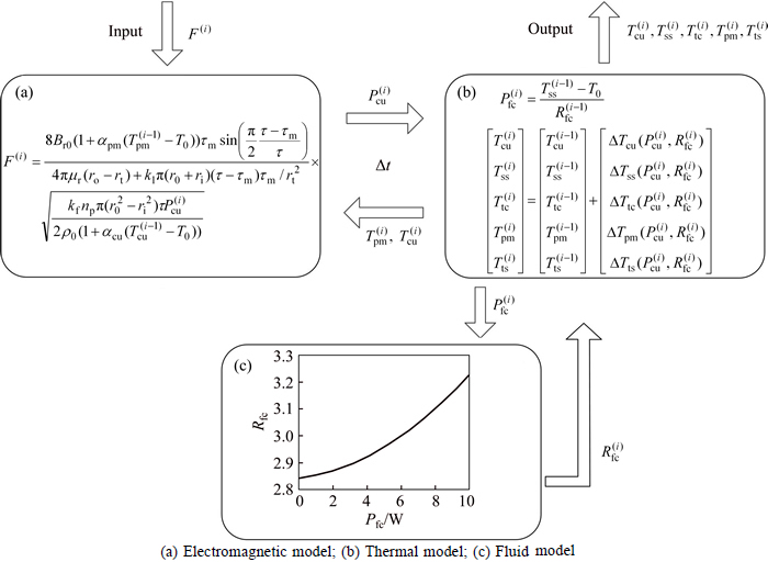
Fig. 5 Transient state analysis based on an iterative computation process:

In the experiment, the ambient temperature is 24 °C. The average thrust force of each TLM is 9 N. The values of the temperature sensors and the infrared camera are recorded every 1 min. Figure6(b) displays the output of the infrared camera at the 5th min, which intuitively displays the temperature differences between different TLMs. Figure7 compares the predicted and the experimental temperature distributions of the 8 TLMs in a row at 5th, 15th and 25th minute respectively. When t= 25 min, the steady state is reached. The corresponding prediction errors are displayed in the right column. It is observed that both the transient state (t=5, 15 min) and the steady state (t=25 min) temperature distributions are accurately predicted. The maximum error is 1.6 °C for predicting the stator surface temperatures and 1 °C for predicting the translator surface temperatures. The errors are primarily caused by the inaccuracy of the fluid modeling especially near the outlet, because the boundary conditions of the actual system are not exactly the same as those of the simulation environment. In addition, the inaccuracy of the lumped-parameter models and the instruments also lead to prediction errors. Though, the temperature prediction accuracy based on the proposed approach is satisfactory for an engineering application. The work contributes to determining a reasonable external load so as to avoid overheating and hence ensuring safety of the radiotherapy machine.

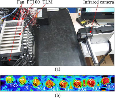
Fig. 6 (a) Experimental setup; (b) Output of infrared camera

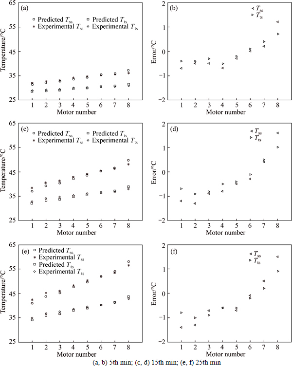
Fig. 7 Comparison of predicted and experimental temperature distributions (a, c, e) and error (b, d, f) of 8 TLMs: (a, b) 5th min; (c, d) 15th min; (e, f) 25th min

6 Conclusions

1) A multi-physics analysis approach is proposed to predict the performance of permanent magnet TLMs under severe volumetric and thermal constraints. This approach considers the coupling effects amongst the electromagnetic and the thermal models of the TLMs as well as the fluid model of the surrounding air, and thereby achieves high computation accuracy.

2) The combined analytical-numerical approach reduces computation cost greatly compared to finite element methods. Specifically, the electromagnetic model based on a lumped-parameter magnetic circuit, the thermal model based on a lumped-parameter thermal network and the fluid model from CFD are incorporated.

3) Both the steady state and the transient state temperature distributions can be predicted in an efficient way. The former is based on analytical equations and the latter is via an iterative computation process. With a study on thermal rating of the TLM under the worst cooling condition, the permissible load is determined to avoid overheating.

4) Experimental measurements of the stator surface and the translator surface temperatures show good consistency with the predicted results.

5) The proposed multi-physics analysis approach can be extended to other electrical machines operating in special environment where the interaction amongst various physical fields is appreciably high.

References

[1] JANG S M, CHOI J Y. Analytical prediction for electromagnetic characteristics of tubular linear actuator with Halbach array using transfer relations [J]. Journal of Electrical Engineering & Technology, 2007, 2(2): 221-230.

[2] MEESSEN K J, PAULIDES J J H, LOMONOVA E A. Modeling and experimental verification of a tubular actuator for 20-g acceleration in a pick-and-place application [J]. IEEE Transactions on Industry Applications, 2010, 46(5): 1891-1898.

[3] WANG J, JEWELL G W, HOWE D. A general framework for the analysis and design of tubular linear permanent magnet machines [J]. IEEE Transactions on Magnetics, 1999, 35(3): 1986-2000.

[4] GYSEN B L J, LOMONOVA E A, PAULIDES J J H, VANDENPUT A J A. Analytical and numerical techniques for solving Laplace and Poisson equations in a tubular permanent-magnet actuator: Part I. Semi-analytical framework [J]. IEEE Transactions on Magnetics, 2008, 44(7): 1751-1760.

[5] BIANCHI N, BOLOGNANI S, CORTE D D, TONEL F. Tubular linear permanent magnet motors: An overall comparison [J]. IEEE Transactions on Industry Applications, 2003, 39(2): 466-475.

[6] LU H, ZHU J, GUO Y. Development of a slotless tubular linear interior permanent magnet micromotor for robotic applications [J]. IEEE Transactions on Magnetics, 2005, 41(10): 3988-3990.

[7] RIDGE A, MATHEKGA M E, CLIFTON P C J, MCMAHON R, KELLY H P. Thermal modelling of a tubular linear machine for marine renewable generation [C]// 6th IET International Conference on Power Electronics, Machines and Drives (PEMD). Bristol, United Kingdom: IET, 2012: B144.

[8] RIDGE A, MCMAHON R, KELLY H P. Detailed thermal modelling of a tubular linear machine for marine renewable generation [C]// IEEE International Conference on Industrial Technology (ICIT). Cape Town, South Africa: IEEE, 2013: 1886-1891.

[9] HUANG X, LIU J, LI L. Calculation and experimental study on temperature rise of a high overload tubular permanent magnet linear motor [J]. IEEE Transactions on Plasma Science, 2013, 41(5): 1182-1187.

[10] SHI Yun-lai, CHEN Chao, ZHAO Chun-sheng. Optimal design of butterfly-shaped linear ultrasonic motor using finite element method and response surface methodology [J]. Journal of Central South University, 2013, 20(2): 393-404

[11] MAKNI Z, BESBES M, MARCHAND C. A coupled electromagnetic-thermal model for the design of electric machines [J]. The International Journal for Computation and Mathematics in Electrical and Electronic Engineering, 2007, 26(1): 201-213.

[12] GUO H, LV Z, WU Z, WEI B. Multi-physics design of a novel turbine permanent magnet generator used for downhole high- pressure high-temperature environment [J]. IET Electric Power Applications, 2013, 7(3): 214-222.

[13] KUMBHAR G B, KULKARNI S V, ESCARELA-PEREZ R, CAMPERO-LITTLEWOOD E. Applications of coupled field formulations to electrical machinery [J]. The International Journal for Computation and Mathematics in Electrical and Electronic Engineering, 2007, 26(2): 489-523.

[14] VESE I C, MARIGNETTI F, RADULESCU M M. Multiphysics approach to numerical modeling of a permanent-magnet tubular linear motor [J]. IEEE Transactions on Industrial Electronics, 2010, 57(1): 320-326.

[15] MEZANI S, TAKORABET N, LAPORTE B. A combined electromagnetic and thermal analysis of induction motors [J]. Transactions on Magnetics, 2005, 41(5): 1572-1575.

[16] ALBERTI L, BIANCHI N. A coupled thermal-electromagnetic analysis for a rapid and accurate prediction of IM performance [J]. IEEE Transactions on Industrial Electronics, 2008, 55(10): 3575- 3582.

[17] WEBB S. Contemporary IMRT: Developing physics and clinical implementation [M]. Bristol, UK: Institute of Physics Publishing, 2005: 1-4.

[18] BOGLIETTI A, CAVAGNINO A, STATON D, SHANEL M, MUELLER M, MEJUTO C. Evolution and modern approaches for thermal analysis of electrical machines [J]. IEEE Transactions on Industrial Electronics, 2009, 56(3): 871-882.

[19] CHURCHILL S W, CHU H H S. Correlating equations for laminar and turbulent free convection from a horizontal cylinder [J]. International Journal of Heat Mass Transfer, 1975, 18(9): 1049-1053.

[20] BARBOSA J R, HERMES C J L, EMLO C. CFD analysis of tube-fin no frost evaporators [J]. Journal of the Brazilian Society of Mechanical Sciences and Engineering, 2010, 32(4): 445-453.

(Edited by FANG Jing-hua)

Foundation item: Project(2015BAI03B00) supported by the National Key Technology R & D Program of China; Project(Z141100000514015) supported by Science and Technology Planning Program of Beijing, China; Project(SKLT12A03) supported by Tribology Science Fund of State Key Laboratory of Tribology, China

Received date: 2015-06-02; Accepted date: 2016-01-18

Corresponding author: YE Pei-qing, Professor, PhD; Tel: +86-10-62773269; E-mail: yepq@tsinghua.edu.cn