J. Cent. South Univ. Technol. (2010) 17: 852-856

DOI: 10.1007/s11771-010-0566-5

Discontinuous flying particle swarm optimization algorithm and its application to slope stability analysis

LI Liang(李亮)^{1, 2}, YU Guang-ming(于广明)¹, CHEN Zu-yu(陈祖煜)², CHU Xue-song(褚雪松)¹

1. School of Civil Engineering, Qingdao Technological University, Qingdao 266033, China;

2. Department of Geotechnical Engineering, China Institute of Water Resources and Hydropower Research,

Beijing 100044, China

? Central South University Press and Springer-Verlag Berlin Heidelberg 2010

Abstract: A new version of particle swarm optimization (PSO) called discontinuous flying particle swarm optimization (DFPSO) was proposed, where not all of the particles refreshed their positions and velocities during each iteration step and the probability of each particle in refreshing its position and velocity was dependent on its objective function value. The effect of population size on the results was investigated. The results obtained by DFPSO have an average difference of 6% compared with those by PSO, whereas DFPSO consumes much less evaluations of objective function than PSO does.

Key words: slope stability; limit equilibrium method; factor of safety; particle swarm optimization

1 Introduction

The slope stability is usually performed by finite element method, limit analysis and limit equilibrium method. At present, numerical methods have been successfully used [1]. However, limit equilibrium method was widely used by the researchers for slope stability analysis because of easy utility and engineering experiences. Although this method did not consider the stress-strain relation of soil, the factor of safety could be estimated without the knowledge of the initial stress conditions and a problem could be defined and solved in a relatively short time. The uses of limit equilibrium for general problems required the selection of trial failure surfaces and minimization of the factor of safety because many proposals were used with success for simple problems.

The complexities of slope stability analyses have drawn the attention of many researchers to find effective and efficient methods for determining the global minimum factor of safety of complex problems. YAMAGAMI and JIANG [2] adopted dynamic programming to determine the critical slip surface. CHEN and SHAO [3] adopted simplex method, steepest descent method and Davidson-Fletcher-Powell method in the conjunction with a grid search solution. GRECO [4] and MALKAWI et al [5] used Monte-Carlo technique to search the critical slip surface. CHENG [6] developed a procedure, which transformed various constraints and requirements of a kinematically acceptable failure mechanism to the evaluation of upper and lower bounds of the control variables and employed simulated annealing algorithm to determine the critical slip surface. ZOLFAGHARI et al [7] utilized genetic algorithm, and BOLTON [8] used leap-frog optimization technique to evaluate the minimum factor of safety. In recent years, there have been other new global optimization methods that are worth considering for application to geotechnical engineering. For example, CHEN et al [9] used particle swarm optimization to locate non-circular slip surfaces of slopes. It was found to be a time consuming algorithm especially for large scale problems. In this work, a modified particle swarm optimization was proposed.

2 Generation of potential slip surfaces

The horizontal distance between x₁ and x_n+1 was subdivided into n equal segments by using

            (1)

where n is the number of slices, the lower and upper bounds to y₂, …, y_n are denoted as y_{2, min}, y_{2, max}, …,   y_{n, min}, y_{n, max}. The solution domains for variables x₁ and x_n+1 can be defined easily by engineering experience, and sufficiently wide domains can be specified by the engineers. As shown in Fig.1, x_i varies between the lower bounds from x_l to x_u and upper bounds from x_L to x_U.

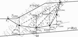
Fig.1 Procedure for generating acceptable slip surface

The procedure for the generation of potential slip surfaces proposed by CHENG [6] was shown in Fig.1. After the values of x₁, …, x_n+1 are given, y_{2, min} and y_{2, max} can be determined by geometry y₁(x) and bed rock line of the slope R(x). y₂ is randomly generated in the range of [y_2min, y_2max]. The line between points V_n+1 and V₂ is intersected with line x=x₃ at point G with y-ordinate y_G, and the line passing through points V₁ and V₂ is extended to intersect with line x=x₃ at point H and y-ordinate y_H is received. y_{3, min} and y_{3, max} are determined by using

                     (2)

y_{4, min}, y_{4, max}, …, y_{n, min}, y_{n, max} are obtained in a way similar to Eq.(2). The slip surface is represented mathematically by vector X=[x₁, x_n+1, y₂, …, y_n]. The number of control variables in this work is m=n+1.

3 Particle swarm optimization (PSO) algorithms

3.1 Sketch of original PSO

PSO algorithm has received wide applications in continuous and discrete optimization problem [10-14]. It is based on the simulation of simplified social models, such as bird flocking, fish schooling, and the swarming theory. In this algorithm, several particles (N particles in total) refer as potential solutions flying in the problem search space to determine their optimum position. This optimum position is usually characterized by the optimum of a fitness function (e.g., factor of safety for the present problem). Each particle is represented by a vector in multi-dimensional space to characterize its position () and another vector to characterize its velocity () at the current time step k. In order to pursue the optimum of the fitness function, velocity  and positionof each particle are adjusted in each time step. The updated velocityis obtained by

       (3)

where i=1, 2, …, N; c₁ and c₂ are responsible for introducing stochastic weighting, which are commonly chosen as 2.0; r₁ and r₂ are random numbers in the range of [0, 1]; w is the inertia weight coefficient, a larger value for w enables the algorithm to explore the search space while a smaller value of w makes the algorithm exploit the refinement of results; O_i is the ith particle’s best position found so far; and O_g is the best position of total group found so far with an objective function of f_g. CHATTERJEE and SIARRY [15] introduced a nonlinear inertia weight variation for dynamic adaptation in PSO.

3.2 Discontinuous flying PSO (DFPSO)

In the present proposal, firstly, algorithms including PSO and DFPSO evolve N₁ iterations, if O_g remains unchanged after N₂ iterations, the algorithm will be terminated. The termination criterion is formulated as follows:

≤                               (4)

where f_sf represents the objective function value of the best solution found so far; and ε is the tolerance of termination, which is chosen as 0.000 1 in this work.

With the increase of the number of slices, i.e., the number of control variables, much more evaluations of objective function are needed by PSO because each particle updates its position by Eq.(3). In order to obtain the optimum solution for the optimization problem within less evaluations of objective function, a new version of PSO (discontinuous flying PSO, DFPSO) was proposed, which is different from PSO in that DFPSO only allows several flies within the whole group of particles. Besides, the particles with better objective function value can fly more time than those with worse objective function value within one iteration. The following flying procedures are adopted.

(1) Several flies instead of one fly are performed for each particle in group. Herein, suppose that N_a≤N flies altogether are allowed in DFPSO in each iteration step. In addition, one particle can fly more than once according to its objective function value. In this work, the better the objective function value of one particle, the more the times it can fly.

A parameter δ (0＜δ＜1.0) is introduced to implement the above procedure, where δ is used to determine the probability of each particle to fly. As there is no theoretical basis for computing δ, δ is randomly generated from 0.2 to 0.5 in this work. The current N particles are sorted by ascending order in terms of objective function values, and the probability of each particle to fly (fly probability) is determined by

               (5)

where p_i is the fly probability of the ith particle. The accumulated probability is represented by array A as follows:

                (6)

A random number r₀ varying from 0 to A(N) is generated. If A(i-1)＜r₀≤A(i), the ith particle will fly once.

(2) After N_a flies are completed, the following procedure for the particles will be checked one by one. If one particle has a chance to fly more than once, it will randomly choose a new position and a new velocity as that in the next iteration and other positions are assigned to those having no chances to fly in the current iteration. The above laws are called the updating rules of DFPSO.

The iterating steps of DFPSO are as follows.

(1) Necessary parameters are initialized as c₁, c₂, w, n, N₁, N₂, f_sf, v_sf, and N_a.

(2) N particles (slip surfaces) are randomly generated, the flying particles and their factors of safety are restored, and O_i and O_g are identified.

(3) The positions and velocities of particles are adjusted by the updating rule described in section 3.2; and N_a flies are performed and one iteration is finished.

(4) If the termination criterion is satisfied, v_sf will be the optimum solution; otherwise, the algorithm will go step (3).

In the following case studies, the common parameters adopted in PSO and DFPSO are: c₁=c₂=2.0, w=0.5, N₁=500, N₂=200. Three different values of N are assumed: 5, m and 2m, where m is the number of control variables. The PSO algorithms are called PSO-1, PSO-2 and PSO-3 respectively regarding the above three different values of N. In the DFPSO, N=2m and N_a=5 are assumed. In addition, the number of evaluated objective functions (N_NOF) is used to represent the time consumed by the algorithm.

4 Case studies

Example 1 was referred to in falls the association for computer aided design (ACAD) study, where there was a 600 mm-thick soft band of soil, and an external vertical load and a water pressure were considered. A referee value of 0.780 0 was recommended as the minimum factor of safety. Table 1 lists the soil parameters. Fig.2 shows the slope profile and layered soils.

It is evident from Table 2 that the PSO-1 falls in the local minimum because only five particles are employed to search the problem space. However, the DFPSO also adjusts five particles’ positions and velocities within one iteration step, obtaining the minimum of 0.725 9 when the number of slices is 40. With the increase of N, the results become superior to those obtained by PSO-1; however, the total N_NOF increases in proportionally. For instance, PSO-3 spends 177 600 evaluations of objective function with the factor of safety of 0.762 6, while DFPSO only uses 8 477 evaluations to find a factor of safety of 0.725 9. The error is nearly up to 6%. As seen from Fig.3, the critical slip surface obtained by DFPSO approaches more closely to the weaker layer than that obtained by others. The average factor of safety of three different slices and the average total N_NOF are calculated according to Table 2 for comparison. The comparison between DFPSO and PSO is demonstrated in Fig.4.

Table 1 Geotechnical parameters of example 1

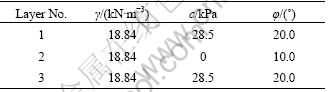
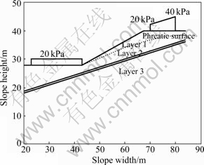
Fig.2 Cross section of example 1

Table 2 Comparison of results between DFPSO and PSO for example 1

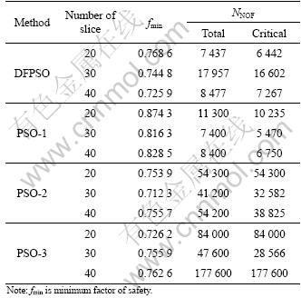
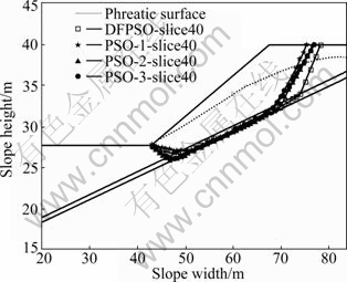
Fig.3 Comparison of critical slip surfaces obtained by different algorithms for example 1

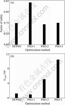
Fig.4 Comparison of average factor of safety (a) and total N_NOF (b) for example 1

Example 2 was a slope in layered soil. The geometric layout of the slope is shown in Fig.5, while Table 3 lists the geotechnical properties for soil layers 1-4, and Table 4 lists comparison of results between DFPSO and PSO for example 2.

It is found that factors of safety lower than those in Ref.[7] are obtained. Although the number of slices used by ZOLFAGHARI et al [7] is not clearly stated, the differences in the factors of safety between the results by the authors in this work and ZOLFGHARI et al [7] are not small, and such differences can be ascribed to different numbers of slices used for computation. Referring to Fig.6, it is noticed that greater portions of the failure surfaces appear within layer 3 as compared with the solution by ZOLFGHARI et al [7]. Hence, lower factors of safety obtained by the authors are more reasonable than those obtained by ZOLFGHARI et al [7].

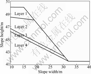
Fig.5 Geometry for example 2

Table 3 Geotechnical parameters for example 2

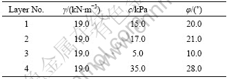
Table 4 Comparison of results between DFPSO and PSO for example 2

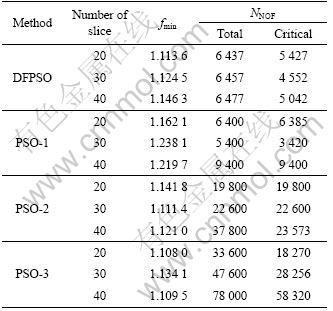
The results obtained by PSO-1 are the worst among the four algorithms, although the total N_NOF used is smaller than that used by DFPSO. The latter algorithm obtains a factor of safety of 1.146 3 for 40 slices, while PSO-3 arrives a factor of safety of 1.110 0 at the cost of 78 000 evaluations. The error is 3.3% between DFPSO and PSO-3. It can be also found from Fig.7 that, compared with PSO-3, DFPSO reaches the minimum factor of safety with less N_NOF.

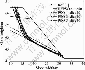
Fig.6 Comparison of critical slip surfaces obtained by ZOLFAGHARI et al [7] and proposed method in this work

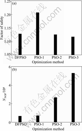
Fig.7 Comparison of average factor of safety (a) and total N_NOF (b) for example 2

5 Conclusions

(1) PSO reaches a global optimum with the increase of the population size and considerably large number of evaluations of objective function.

(2) DFPSO solves the problem with the error range smaller than 6% compared to PSO with larger population size, while DFPSO only consumes approximately 10 000 evaluations of objective function value. So DFPSO can be used to solve complex optimization problems.

References

[1] YANG Xiao-li, SUI Zhi-rong. Seismic failure mechanisms for loaded slopes with associated and nonassociated flow rules [J]. Journal of Central South University of Technology, 2008, 15(2): 276-279.

[2] YAMAGAMI T, JIANG J C. A search for the critical slip surface in three-dimensional slope stability analysis [J]. Soils and Foundations, 1997, 37(3): 1-16.

[3] CHEN Z, SHAO C. Evaluation of minimum factor of safety in slope stability analysis [J]. Canadian Geotechnical Journal, 1988, 25(4): 735-748.

[4] GRECO V R. Efficient Monte Carlo technique for locating critical slip surface [J]. Journal of Geotechnical Engineering, 1996, 122(3): 517-525.

[5] MALKAWI A I H, HASSAN W F, SARMA S K. Global search method for locating general slip surface using Monte Carlo techniques [J]. Journal of Geotechnical and Geoenvironmental Engineering, 2001, 27: 688-698.

[6] CHENG Y M. Location of critical failure surface and some further studies on slope stability analysis [J]. Computers and Geotechnics, 2003, 30(3): 255-267.

[7] ZOLFAGHARI A R, HEATH A C, MCCOMBIE P F. Simple genetic algorithm search for critical non-circular failure surface in slope stability analysis [J]. Computers and Geotechnics, 2005, 32(3): 139-152.

[8] BOLTON H P J, HEYMANN G, GROENWOLD A. Global search for critical failure surface in slope stability analysis [J]. Engineering Optimization, 2003, 35(1): 51-65.

[9] CHEN Yun-min, WEI Xin-jiang, LI Yu-chao. Locating non-circular critical slip surfaces by particle swarm optimization algorithm [J]. Chinese Journal of Rock Mechanics and Engineering, 2006, 25(7): 1443-1449. (in Chinese)

[10] YIN P Y. A discrete particle swarm algorithm for optimal polygonal approximation of digital curves [J]. Journal of Visual Communication and Image Representation, 2004, 15(2): 241-260.

[11] PAN Q K, TASGETIREN FAITH M, LIANG Y C. A discrete particle swarm optimization algorithm for the no-wait flowshop scheduling problem [J]. Computers and Operations Research, 2008, 35(9): 2807-2839.

[12] LIAO C J, TSENG C T, LUARN P. A discrete version of particle swarm optimization for flowshop scheduling problems [J]. Computers and Operations Research, 2007, 34(10): 3099-3111.

[13] ESQUIVEL SUSANA C, COELLO CARLOS A. Hybrid particle swarm optimizer for a class of dynamic fitness landscape [J] Engineering Optimization, 2006, 38(8): 873-888.

[14] SURIBABU C R, NEELAKANTAN T R. Design of water distribution networks using particle swarm optimization[J]. Urban Water Journal, 2006, 3(2): 111-120.

[15] CHATTERJEE A, SIARRY P. Nonlinear inertia weight variation for dynamic adaption in particle swarm optimization [J]. Computers and Operations Research, 2006, 33(3): 859-871.

Foundation item: Project(50874064) supported by the National Natural Science Foundation of China; Key Project(Z2007F10) supported by the Natural Science Foundation of Shandong Province, China

Received date: 2009-10-08; Accepted date: 2010-01-27

Corresponding author: LI Liang, PhD, Associate professor; Tel: +86-532-85071278; E-mail: liangli14@yahoo.com.cn

(Edited by CHEN Wei-ping)