Trans. Nonferrous Met. Soc. China 24(2014) 224-232

Contrast between 2D inversion and 3D inversion based on 2D high-density resistivity data

De-shan FENG^1,2, Qian-wei DAI^1,2, Bo XIAO^1,2

1. School of Geosciences and Info-Physics, Central South University, Changsha 410083, China;

2. Key Laboratory of Metallogenic Prediction of Nonferrous Metals, Ministry of Education, Changsha 410083, China

Received 30 December 2012; accepted 27 April 2013

Abstract: The 2D data processing adopted by the high-density resistivity method regards the geological structures as two degrees, which makes the results of the 2D data inversion only an approximate interpretation; the accuracy and effect can not meet the precise requirement of the inversion. Two typical models of the geological bodies were designed, and forward calculation was carried out using finite element method. The forward-modeled profiles were obtained. 1% Gaussian random error was added in the forward models and then 2D and 3D inversions using a high-density resistivity method were undertaken to realistically simulate field data and analyze the sensitivity of the 2D and 3D inversion algorithms to noise. Contrast between the 2D and 3D inversion results of least squares inversion shows that two inversion results of high-density resistivity method all can basically reflect the spatial position of an anomalous body. However, the 3D inversion can more effectively eliminate the influence of interference from Gaussian random error and better reflect the distribution of resistivity in the anomalous bodies. Overall, the 3D inversion was better than 2D inversion in terms of embodying anomalous body positions, morphology and resistivity properties.

Key words: high-density resistivity method; finite element method; forward simulation; least square inversion; 2D inversion; 3D inversion; apparent resistivity

1 Introduction

High-density resistivity data sets can be collected in combination with a variety of other field data techniques. The accuracy of such data sets is often high because a large amount of information is collected. Excellent geological constraints are widely used and recognized as part of engineering investigations [1], regional geological surveys [2] and other field campaigns. High-density resistivity has become one of the most popular geophysical techniques for the fast mapping of large areas prospecting. Many common geophysical inversion methods are widely used to process and interpret high-density resistivity data to get higher exploration precision and to more intuitively interpret profiles. These include the nonlinear inversion method and linear inversion method. WANG et al [3] used the least square method to enhance sharp boundary in multi-electrode resistivity sounding. MUKANOVA and ORUNKHANOV [4] studied the conjugate gradient method (CGM) inverse resistivity problem: geoelectric uncertainty principle and numerical reconstruction method. RODI and MACKIE [5] applied the non-linear conjugate gradients algorithm for 2D magnetotelluric inversion. MUIUANE and PEDERSEN [6] processed the 1D inversion of DC resistivity data using a quality-based truncated SVD. LOKE and DAHLIN [7] contrasted the Gauss-Newton and quasi-Newton methods in resistivity imaging inversion. SHASHI [8] compiled a very fast simulated annealing FORTRAN program for interpretation of 1D DC resistivity sounding data from various electrode arrays. In order to solve the problem that the solution of the traditional local linear iterative inversion is likely to fall into the local minimum solution and rely on the choice of initial model, MA et al [9] applied BP neural network to calculating high-density electrical resistivity. However, many data translators are often restricted to 2D high-density electrical resistivity inversion algorithms. That is, they treat geological structures as 2D bodies for 2D inversion [10,11], even though most geological structures are actually 3D bodies. Therefore, 2D inversion results are only approximate [12] and the determination of the calculation accuracy is difficult to achieve. This leads to the practical significance of advancing research in 3D inversion methods [13-15]. JACKSON et al [16] utilized a 3D resistivity inversion algorithm on 2D measured data and obtained good results. HUANG and RUAN [17] took a large number of high-density resistivity simulation experiments, and illustrated that 3D inversion techniques are better than 2D inversion for determining abnormal position, morphology and resistivity properties.

Optimal 3D inversion of high-density resistivity data is based on 3D data acquisition, but such raw 3D data sets often cannot be easily obtained in practical exploration setting due to economic and field logistic factors. Therefore, most field exploration is still based on 2D data acquisition, so developing suitable methods that use 2D data in 3D inversions is very important. This work starts with a discussion of 2D and 3D inversion theory, and carries out 2D and 3D inversions on two typical geological body models and an engineering field test datum. The results show that the 3D inversion is affected only slightly by Gaussian random error, and is better than the 2D inversion in determining unusual position. Therefore, 3D inversion is more accurate.

2 2D and 3D resistivity forward modeling and inversion characteristics

Although an improved inversion is the ultimate goal, the forward simulation is the key of 2D and 3D inversion [18]. In this work, the finite element method is adopted for forward simulations. The calculation space is divided into a grid of interconnected unit cells. The potential distribution of the computational domain can be obtained by solving for the potential of unit grid nodes. Then, the potential distribution values are converted into apparent resistivity values. 3D resistivity forward models address 3D problems in a 3D field. This means that the sets of 3D differential equations are satisfied at all nodes of a stable 3D current field generated by a point power supply. The boundary value problem of the 3D differential equation is satisfied by the potential function U=U(x, y, z) as follows:

(1)

where,

2D resistivity forward modeling can refer to the study on a 2D problem in a 3D field where the conductivity of a subsurface medium has no change along one direction (e.g., the y-axis direction). A cosine Fourier transform is carried out on the 3D partial differential equation (PDE) satisfied by the potential function of a stable 3D current field generated by a point power supply; this thereby changes a 3D PDE into a 2D PDE. Under 2D conditions, the calculation of all node of the point source current field can be attributed to a boundary value problem of a 2D PDE satisfied with the Fourier transform V(x, λ, z):

              (2)

where

σ is the conductivity; Γ_s and Γ₁ are the ground boundaries; Γ_∞ is the other boundary; I_k refers to the current intensity of the kth current electrode; r is the distance between field source and measuring point; n refers to the boundary normal vector; and K₀(λr_k) and K₁(λr_k) respectively refer to the zero-order and one-order modified Bethesda Seoul functions.

The variational problem equivalent to Eq. (1) is as follows:

    (3)

The solution of Eq. (3) can determine the potential U(x, y, z) for all grid nodes in a 3D earth current cross section.

The variational problem equivalent to Eq. (2) is as follows:

 (4)

The solution of Eq. (4) can determine the transform potential V(x, y, z). The Fourier inverse transform is then carried out:

                   (5)

thereby calculating potential values of all grid nodes of the 2D earth current cross section. The objects and processes of 2D and 3D forward simulations have certain differences, so in turn the inversion results are also different.

The 2D and 3D resistivity-method inversion processes adopted by this work are consistent. They are based on the least squares principle, and utilize forward modeling of measured data to minimize a constructed objective function [19]. The objective function, Φ, of the least squares inversion problems [20] can be expressed as

                            (6)

In the formula,

and J refers to the partial derivative matrix; m is an N-dimensional model vector; d is the M-dimensional measured apparent resistivity vector; m_i is the ith model parameter, ⁰ represents the partial derivative of the primary model m₀ on the jth observation value d_i to the ith model parameter m_i; △m=m-m⁰ is the model parameter modified vector; △d=d-d⁰ is the data residuals vector, namely, the difference of the logarithm of the measured apparent resistivity and the logarithm of the simulated apparent resistivity.

Traditional damped least square inversion models generate excess construction [21] because the inverse model parameters have more relative measured data. In the 2D or 3D resistivity inversion process, a smooth matrix constraint can be added to the inverse objective function. The physical meaning of such a condition is to make the subsurface model as smooth and as simple as possible. Mutations in the resistivity model among adjacent grids can then be reduced, thereby reducing the number of possible inverse solutions. The objective function Eq. (6) is modified with smoothing constraints as follows:

              (7)

The objective function containing the smoothing constraints is differentiated on △m, and is made to be equal to 0. Linear equations can be obtained:

            (8)

where l is the Lagrange multiplier and C is a smoothing matrix. The model parameter modification vector △m can be obtained by solving Eq. (8), which is substituted into the following formula:

                           (9)

A new forecasting model parameter vector m^(k) will be obtained. This process is repeated until the root mean square (RMS) error between the measured and simulated data satisfies requirements. At this point, the resistivity inversion process is complete.

                          (10)

3 Model calculation and inversion

3.1 High-resistance body model

The anomalous body adopted for the data simulation was a high impedance cube with side length of 3 m. The cube had a resistivity of 100 Ω×m and the resistivity of the surrounding rock was 50 Ω×m. The simulated domain covered a volume measured of 10 m×10 m×7 m region with the anomalous body located at its center and the top of the cube buried 0.7 m below the top of the domain (Fig. 1). Data acquisition used the pole-pole arrangement, with 11 survey lines arranged over the simulated domain. Each survey line consisted of 11 potential electrodes, resulting in a total deployment of 121 electrodes. Station and line spacings were both 1 m (Fig. 1). Following the finite element method forward calculation, apparent resistivities were contoured. This process was repeated after 1% Gaussian random error was added to more closely simulate real-world conditions. The results enable the sensitivity of high-density 2D and 3D resistivity data inversions (with noise) to be analyzed.

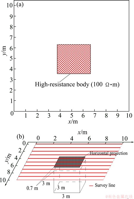
Fig. 1 2D plane view map (a) and 3D spatial sketch map (b) of high-resistance body model

Forward-modeled data containing Gaussian random error were used for the high-density 2D resistivity method inversion. Inversion results from the same depth were extracted and combined into horizontal slice maps through interpolation (Figs. 2(a₁-a₆)). The mean was selected for inversion results of adjacent survey lines, thereby forming a vertical slice map mid-way between neighboring survey lines in the x-direction. The adjacent region of the anomalous body was selected for slicing (Figs. 3(a₁-a₆)). The process was repeated for the high- density 3D resistivity method inversion. The 3D results were sliced horizontally at the same depth as done previously for the 2D inversion (Figs. 2(b₁-b₆)). x-direction vertical slicing was carried out on the inversion results near the anomalous body (Figs. 3(b₁-b₆)).

Fig. 2 Horizontal slice maps of high resistance body model inversion result at different depths

A comparison of Figs. 2 and 3 shows that the 2D and 3D inversion results of high-density resistivity method can basically reflect the spatial position of an anomalous body. However, both 2D and 3D images can represent anomalous subsurface features to a greater or lesser extent. 2D inversion was greatly influenced by Gaussian random error. In our example, the slices through the inversion results on either side of the anomalous body had poor symmetry; the anomaly seen on the model slices is not particularly good as it is known that the anomalous body had a regular spatial structure. The inversion results contained greater errors in the analysis of the practical position and resistivity of the anomalous body where h=-3 m on the horizontal slice map (Fig. 2(a₄)) and y=3.5 or 6.5 m slice maps (Figs. 3(a₂, a₅)). In contrast, 3D inversion was little affected by the presence of Gaussian random errors, and realistically reflected the known shape structure and resistivity distribution of the test body. The corresponding slice maps through the inverted model on both sides of the anomalous body had good symmetry. All slice maps embodied good axial symmetry, and showed that the anomalous body was a symmetric structure.

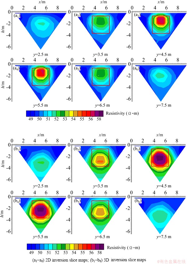
Fig. 3 Vertical slice maps of high resistance body model inversion result in x-direction

3.2 Composite model

A model containing a combination of high and low resistivities was selected for a second forward simulation. Again, 2D and 3D inversions were carried out on forward-modeled apparent resistivity sections, and the 2D and 3D inversion results determined from 2D high-density data were compared. The numerical simulation used a 3 m × 3 m × 2.5 m high-resistance (100 Ω×m) block and a 3 m × 3 m × 3 m low-resistance (10 Ω×m) cube. The resistivity of the surrounding rock was 50 Ω×m. The simulated domain was 13 m × 8 m × 10 m in extent, with the depth to the top of the high-resistance block at 0.7 m and the depth to the top of the low-resistance cube at 1.2 m. Data acquisition again used the pole-pole arrangement with 9 survey lines, and each contained 14 electrodes arranged over the simulated domain. In all, 126 electrodes were positioned with the station and line spacing both being 1 m (Fig. 4).

The inversion results are displayed as both cross sections (Figs. 5(a₁-a₉)) and horizontal slice maps (Figs. 6(a₁-a₆)) through interpolation. Similarly, the forward-modeled data from the region were integrated for a high-density 3D resistivity method inversion. The inversion results in this case were 3D structures. Invalid inversion data were removed, and vertical (Figs. 5(b₁-b₉)) and horizontal (Figs. 6(b₁-b₆)) slices were obtained through the 3D inversion at the same positions and depths. Figures 5 and 6 show that both the 2D and 3D high-density resistivity method inversions reflect the same basic spatial positions of the anomalous bodies. All slice maps embody the connectivity of the anomalies to a greater or lesser extent and high- and low-resistance anomaly decomposition regions were obvious.

However, the 2D inversion was greatly affected by Gaussian random error, resulting in more false anomalies. The inversion result slice maps on the two sides of the anomalous bodies had poorer symmetry, and the low-resistivity anomalous body in the inversion results had greater errors from the actual location and resistivity in model II. The 3D inversion was little affected by Gaussian random error, and the anomalous body shape structure and resistivity distribution can be reflected more realistically. The low-resistance feature and practical anomalous body position in the 3D inversion model corresponded well. The anomalous body’s shape had no prominent changes corresponding to the horizontal depth. The corresponding inversion result slice maps on both sides of the anomalous bodies were symmetric; in fact, all slice maps embodied good axis symmetry, which indicated that the anomalous bodies were regular symmetrical structural bodies in 3D.

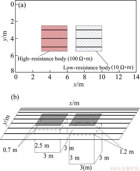
Fig. 4 2D plane view map (a) and 3D spatial sketch map (b) of composite model

Comprehensive analysis of 2D and 3D inversion effects on the two geoelectricity models shows that the connectivity of the anomalous bodies in neighboring slices of the high-density 3D inversion results was better than that of the 2D inversion results. The 3D inversion can more effectively eliminate the influence of interference from Gaussian random error and better reflect the distribution of resistivity in the anomalous bodies. Over all, the 3D inversion was better than 2D inversion in terms of embodying anomalous body positions, morphology and resistivity properties.

4 Conclusions

1) The 2D and 3D inversion results of two typical geoelectricity theory models were successfully compared. It was found that 3D inversion is mostly unaffected by Gaussian random errors. Also, the inversion results are better than for 2D inversion in identifying and characterizing abnormal position, morphology and resistivity properties.

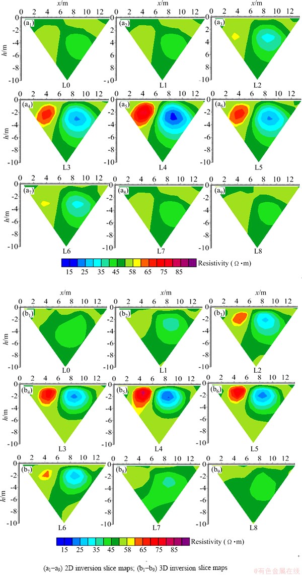
Fig. 5 Vertical slice maps of composite model inversion result in x-direction

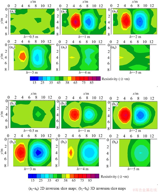
Fig. 6 Horizontal slice maps of composite model inversion result at different depths

2) Compared with multiple 2D inversions that treat the objective body as 2D, the 3D inversion based on 2D high-density resistivity exploration data treating the objective body as a 3D cube has a better calculation accuracy and its inversion effect is slighter. This makes the 3D method more practical and effective.

References

[1] RUCKER D F, LEVITT M T, GREENWOOD W J. Three-dimensional electrical resistivity model of a nuclear waste disposal site [J]. Journal of Applied Geophysics, 2009, 69: 150-164.

[2] RINGS J, HAUCK C. Reliability of resistivity quantification for shallow subsurface water processes [J]. Journal of Applied Geophysics, 2009, 68: 404-416.

[3] WANG Hao, YU Peng, XIANG Yang. An inversion method to enhance sharp boundary in multi-electrode resistivity sounding [J]. Chinese Journal of Engineering Geophysics, 2012, 9: 516-521. (in Chinese)

[4] MUKANOVA B, ORUNKHANOV M. Inverse resistivity problem: Geoelectric uncertainty principle and numerical reconstruction method [J]. Mathematics and Computers in Simulation, 2010, 80: 2091-2108.

[5] RODI W, MACKIE R L. Non-linear conjugate gradients algorithm for 2-D magnetotelluric inversion [J]. Geophysics, 2001, 66: 174-187.

[6] MUIUANE E A, PEDERSEN L B. 1-D inversion of DC resistivity data using a quality-based truncated SVD [J]. Geophysical Prospecting, 2001, 49: 387-394.

[7] LOKE M H, DAHLIN T. A comparison of the Gauss-Newton and quasi-Newton methods in resistivity imaging inversion [J]. Journal of Applied Geophysics, 2002, 49: 149-162.

[8] SHASHI P S. VFSARES-A very fast simulated annealing FORTRAN program for interpretation of 1-D DC resistivity sounding data from various electrode arrays [J]. Computers & Geosciences, 2012, 42: 177-188.

[9] MA Bin, MA Yan-shuang, WANG Yong-hui, BIAN Yan-li, ZHANG Wan-jiang, GUO Tong-ying. High-density resistivity data inversion method based on BP neural network [J]. Journal of Shenyang Jianzhu University: Natural Science, 2010, 26: 599-603. (in Chinese)

[10] LOKE M H, ACWORTH I, DAHLIN T. A comparison of smooth and blocky inversion methods in 2D electrical imaging surveys [J]. Exploration Geophysics, 2003, 34: 182-187.

[11] BOONCHAISUK S, VACHIRATIENCHAI C, SIRIPUNVARA- PORN W. Two-dimensional direct current (DC) resistivity inversion: Data space Occam's approach [J].Physics of the Earth and Planetary Interiors, 2008, 168: 204-211.

[12] ZHOU B, DAHLIN T. Properties and effects of measurement errors on 2D resistivity imaging surveying [J]. Near Surface Geophysics, 2003, 1: 105-117.

[13] GARETH J, MARCIN Z, PHILIPPE S. Mapping desiccation fissures using 3-D electrical resistivity tomography [J]. Journal of Applied Geophysics, 2012, 84: 39-51.

[14] MARIANA A, GIOVANNI B, ROBERTA R, A G, STELLA L, J F G. Multi-electrode 3D resistivity imaging of alfalfa root zone [J]. European Journal of Agronomy, 2009, 31: 213-222.

[15] HU Wen-zhi, MA Hai-tao, XIE Zhen-hua, LI Quan-ming. Application of three dimensional high-density resistivity method in hidden danger detection of tailings [J]. Journal of Safety Science and Technology, 2011, 7: 64-67. (in Chinese)

[16] JACKSON P D, EARL S J, REECE G J. 3D resistivity inversion using 2D measurements of the electric field [J]. Geophysical Prospecting, 2001, 49: 26-39.

[17] HUANG Jun-ge, RUAN Bai-yao. An analytical comparison between 2D and 3D inversions in DC resistivity sounding [J]. Geophysical & Geochemical Exploration, 2004, 28: 447-450. (in Chinese)

[18] DAI Qian-wei, XIAO Bo, FENG De-shan, LIU Hai-fei, WANG Peng-fei. 3-D inversion of high density resistivity method based on 2-D exploration data and its application [J]. Journal of Central South University: Science and Technology, 2012, 43: 293-300. (in Chinese)

[19] MURAT B, LEYLA S. Two-dimensional resistivity imaging in the Kestelek boron area by VLF and DC resistivity methods [J]. Journal of Applied Geophysics, 2012, 82: 1-10.

[20] VIKAS C B, ANTJE F, RALPH-UWE B, KLAUS S. Unstructured grid based 2-D inversion of VLF data for models including topography [J]. Journal of Applied Geophysics, 2011, 75: 363-372.

[21] SMITH J T, BOOKER J R. Magnetotelluric inversion for minimum structure [J]. Geophysics, 1998, 53(12): 1565-1576.

基于二维高密度电阻率数据的二、三维反演对比

冯德山^1,2，戴前伟^1,2，肖 波^1,2

1. 中南大学 地球科学与信息物理学院，长沙 410083；

2. 有色金属成矿预测教育部重点实验室，长沙 410083

摘  要：目前高密度电阻率法所采用的数据处理方法主要是将地质结构体视为二度体进行二维处理，因而二维数据资料处理结果只是一种近似解释，其计算精度与反演效果达不到精确反演的要求。设计两种典型的电阻率异常地质体模型，利用有限单元法进行正演计算。为更真实地模拟实测数据并分析二维、三维反演算法对噪声的敏感度，在正演剖面中加入1%的高斯随机误差，然后再分别利用最小二乘法进行高密度电阻率法二维、三维反演。对比二维和三维高密度电阻率法的反演水平切片及垂直切片图可知，三维反演受高斯随机误差的影响更小，反演结果在模型异常位置、形态和电阻率特性反映上都比二维反演的效果更好，与实际地质模型更接近。

关键词：高密度电阻率法；有限单元法；正演模拟；最小二乘反演；二维反演；三维反演；视电阻率

(Edited by Sai-qian YUAN)

Foundation item: Projects (41074085, 41374118) supported by the National Natural Science Foundation of China; Project (20120162110015) supported by Doctoral Fund of Ministry of Education of China; Project (NCET-12-0551) supported by Program for New Century Excellent Talents in University, China

Corresponding author: Qian-wei DAI; Tel: +86-731-88836456; E-mail: qwdai@csu.edu.cn

DOI: 10.1016/S1003-6326(14)63051-X