Trans. Nonferrous Met. Soc. China 31(2021) 125-137

Estimation of wear performance of AZ91 alloy under dry sliding conditions using machine learning methods

Fatih AYDIN¹, Rafet DURGUT²

1. Department of Metallurgical and Materials Engineering, Karabuk University, Karabuk, Turkey;

2. Department of Computer Engineering, Karabuk University, Karabuk, Turkey

Received 16 March 2020; accepted 1 December 2020

Abstract: The wear behavior of AZ91 alloy was investigated by considering different parameters, such as load (10-50 N), sliding speed (160-220 mm/s) and sliding distance (250-1000 m). It was found that wear volume loss increased as load increased for all sliding distances and some sliding speeds. For sliding speed of 220 mm/s and sliding distance of 1000 m, the wear volume losses under loads of 10, 20, 30, 40 and 50 N were calculated to be 15.0, 19.0, 24.3, 33.9 and 37.4 mm³, respectively. Worn surfaces show that abrasion and oxidation were present at a load of 10 N, which changes into delamination at a load of 50 N. ANOVA results show that the contributions of load, sliding distance and sliding speed were 12.99%, 83.04% and 3.97%, respectively. The artificial neural networks (ANN), support vector regressor (SVR) and random forest (RF) methods were applied for the prediction of wear volume loss of AZ91 alloy. The correlation coefficient (R²) values of SVR, RF and ANN for the test were 0.9245, 0.9800 and 0.9845, respectively. Thus, the ANN model has promising results for the prediction of wear performance of AZ91 alloy.

Key words: AZ91 alloy; wear performance; artificial neural networks; support vector regressor; random forest method

1 Introduction

Magnesium (Mg) is a promising material due to its low density and high specific strength for aerospace and automotive industry [1]. However, the poor mechanical, wear and corrosion properties make it challenging to use in the industrial applications [2]. In order to deal with the disadvantages of Mg, different alloys have been used for many years [3]. Among a variety of Mg alloys, AZ91 is one of the most common alloys with good castability, machinability and corrosion resistance [4].

Even though Mg alloys are not suitable for bearing and gear materials, it is possible that their surfaces may contact with different materials [5]. Wear is one of the most critical and important issues that reduce service life. Therefore, a systematic examination of the tribological behavior of Mg alloys has the critical importance [6].

There have been many studies regarding the wear behavior of AZ91 alloy [1,6-8]. In one of those studies, CHEN and ALPAS et al [7] investigated the wear properties of AZ91 alloy under dry sliding conditions. They observed that there were two regimes as mild and severe. In the mild wear regime, two wear mechanisms were observed (oxidation and delamination). As for the severe regime, melt wear due to severe plastic deformation was observed. SHANTHI et al [1] investigated the effect of grain size on the wear behavior of AZ91D alloy under low sliding speed conditions. In this study, at a sliding speed of less than 0.1 m/s, abrasive wear was identified as a dominant mechanism. They also reported that the wear rate was significantly reduced due to the presence of protective oxidized debris.

Delamination was seen as the dominant mechanism for sliding speed of 0.5 m/s. ZAFARI et al [6] studied the tribological behavior of AZ91D alloy at elevated temperatures. Under a load of 40 N, severe plastic deformation possessed wear at 100 °C and above. When temperature increased to 250 °C, the wear rate decreased. The reduction in wear rate at elevated temperatures was attributed to the oxide formation. WANG et al [8] analyzed the sliding wear properties of AZ91D alloy at 25, 100 and 200 °C. It was concluded that AZ91 alloy exhibited a lower wear rate at 200 °C compared to 25 and 100 °C under loads of 12.5-25 N. At loads of 100, 200 and 250 N, a transition from mild wear regime to severe wear regime was observed with increasing load at 25, 100 and 200 °C. From the above literature studies, it is understood that researchers generally focused on the dry sliding tribological performance of AZ91 alloy for different loads, sliding speeds and test temperatures. All these studies were only experimental studies. The aim of these literature studies was to evaluate the wear mechanisms and wear transitions under different wear conditions.

It is possible to observe many studies concerning wear behavior of AZ91 alloy at room and elevated temperatures under dry sliding conditions. To the best of our knowledge, there are limited number of studies concerning wear behavior using machine learning techniques. In one of those studies, VIGNESH and PADMANABAN et al [9] estimated the tribological properties of wrought AZ91 alloy using artificial neural network (ANN) and Sugeno-Fuzzy logic methods. It was concluded that Sugeno-Fuzzy logic method had the highest accuracy for predicting wear rate compared to ANN.

Machine learning methods are widely used in many disciplines to classify and predict different properties of materials [10]. Among these methods, ANN, support vector regressor (SVR) and random forest (RF) are the most commonly used algorithms [11]. By using these methods, different properties of materials such as specific wear rate [12], tool wear [13] and tensile strength [14] can be estimated with high accuracy. Unlike deep learning that requires a high amount of training data sets, ANN, SVR and RF algorithms can estimate the characteristics of engineering materials with high accuracy, even if the number of training data sets is too small [15-17].

In the present study, the dry sliding wear behavior of AZ91 alloy was investigated by reciprocating wear tests. The wear behavior was studied under different loads, sliding speeds and sliding distances. In order to clarify the wear mechanisms, worn surfaces and wear debris were examined by scanning electron microscopy (SEM). ANN, SVR and RF models were used to estimate the wear volume loss of AZ91 alloy. ANOVA was also used to find the contribution of each parameter on the wear volume loss.

2 Experimental

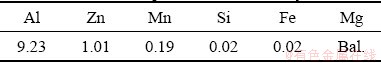
In this study, AZ91 alloy was used for wear tests. The chemical composition of this alloy was given in Table 1. Hardness tests were carried out  on the hardness device (Qness, Q10 A⁺). Five successful measurements were performed at a load of 5 N for 15 s and the mean value was calculated to determine the hardness value of the sample. The hardness of the AZ91 alloy was (73.7±2.1) HV_5 N.  The microstructure examination of the AZ91 alloy was performed by SEM (Carl Zeiss Ultra Plus). The phase analysis of the AZ91 alloy was performed using X-ray diffractometer (Rigaku Ultima IV). Diffraction patterns were obtained over a range of 2θ angles from 20° to 80°.

Table 1 Chemical composition of AZ91 alloy (wt.%)

Figures 1(a) and (b) show the SEM image and XRD pattern of the AZ91 alloy, respectively. Interdendritic β-Mg₁₇Al₁₂ eutectic (white area) with irregular morphology can be seen in α-Mg matrix (dark grey area). It is also observed that the β-Mg₁₇Al₁₂ phase with lamellar morphology is close to the irregular β-Mg₁₇Al₁₂ phase. The formation of the lamellar β-Mg₁₇Al₁₂ phase is related to the cooling after solidification by cellular  precipitation [6]. Solidification of the AZ91 alloy was reported to begin the nucleation of α-Mg dendrites followed by the formation of the β-Mg₁₇Al₁₂ when temperature is close to 437 °C [18]. The presence of similar phases in the AZ91 alloy has been reported in Refs. [6,19]. XRD results also confirmed the presence of α-Mg and β-Mg₁₇Al₁₂ phases in the structure of the AZ91 alloy (Fig. 1(b)).

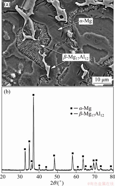
Fig. 1 SEM micrograph (a) and XRD pattern (b) of AZ91 alloy

Dry sliding wear tests were performed by the reciprocating wear tester (UTS, T10/T20). AISI 52100 steel was used as a counterface material. Wear test samples were ground with SiC papers (240-2000 grit size) and polished with diamond solution. The surfaces of the samples were cleaned with alcohol before each test. The wear tests were performed at sliding speeds of 160, 180, 200 and 220 mm/s and loads of 10, 20, 30, 40 and 50 N.  The sliding distances were 250, 500 and 1000 m. The friction coefficient and wear depth values were obtained from reciprocating wear tester simultaneously. Table 2 shows the wear test conditions for this study. The wear volume loss was calculated using wear depth, wear width and stroke distance. Wear width was measured with a digital microscope (Nikon ShuttlePix). Volume loss (mm³) was calculated as the volume area (mm²) multiplied by the stroke distance.

The worn surfaces and wear debris were examined by SEM (Carl Zeiss Ultra Plus) equipped with an energy-dispersive spectrometer EDS (Bruker X Flash 6/10) so as to clarify the wear mechanisms.

Table 2 Wear test parameters of test specimen AZ91 alloy

3 Results and discussion

3.1 Friction coefficient and wear volume loss

Figure 2 illustrates the average friction coefficients (AFCs) of the AZ91 alloy as a function of the sliding speed, load and sliding distance. The AFC graph at sliding distance of 250 m is given in Fig. 2(a). It was seen that the maximum value of AFC was obtained under load of 10 N for all sliding speeds. AFC values decreased in the transition of load from 10 to 20 N. The decrease in AFC is attributed to the oxide formation due to frictional heat produced during sliding motion [4]. The upward trend of AFC was observed under a load of 30 N. The sudden increase is mainly associated with transmitted shear strain [4]. At a sliding distance of 250 m, the AFC was calculated between 0.230 and 0.195. Figure 2(b) depicts the AFC graph at a sliding distance of 500 m. It was seen that AFC fluctuated between 0.215 and 0.235. A decreasing tendency of AFC was observed except for sliding speed of 220 mm/s in the load transition of load from 10 to 20 N. A sharp increase was observed for sliding speed of 220 mm/s in the transition of load from 40 to 50 N. Figure 2(c) illustrates the AFC graph at a sliding distance of 1000 m. Initially, the AFC generally decreased at loads from 10 to 20 N except for that at a sliding speed of 180 mm/s and then showed an increase trend at loads from 20 to 30 N. At a sliding speed of 160 mm/s, AFC dropped from 0.25 to 0.23 in the transition of load from 30 to 40 N. It was generally seen that AFC values were not stable at different loads, sliding speeds and sliding distances. Differences in AFC values are generally associated with different wear mechanisms [20].

Fig. 2 Average friction coefficients of AZ91 alloy at different sliding distances

Fig. 3 Wear volume loss values of AZ91 alloy at different sliding distances

Figure 3 shows the wear volume loss of the AZ91 alloy depending on sliding speed, applied load and sliding distance. From the graphs, it was concluded that wear volume loss of the AZ91 alloy significantly changed depending on load, sliding distance and sliding speed. The variation in wear volume loss is shown in Fig. 3(a) at a sliding distance of 250 m. It was seen that wear volume loss increased with increasing load at all sliding speeds. The lowest wear volume loss was obtained at a sliding speed of 220 mm/s under all loads except for a load of 50 N. At a sliding speed of 200 mm/s, a sharp increase in wear volume loss was observed in the load transition from 10 to 30 N. Under higher loads (30, 40 and 50 N), the highest wear volume loss was calculated at this sliding speed. The wear volume loss at a sliding distance of 500 m was plotted against load as shown in Fig. 3(b). The minimum wear volume loss was obtained at a sliding speed of 220 mm/s. As expected, wear volume loss increased as load increased. It can be inferred from Fig. 3(b) that the rate of increase in wear volume loss generally decreased at loads above 20 N. Figure 3(c) presents the wear volume loss at a sliding distance of 1000 m. The lowest wear volume loss was achieved at a sliding speed of 200 mm/s up to a load of 30 N. At loads higher than 30 N, the wear volume loss at a sliding speed of 160 mm/s had the lowest wear volume loss. These results showed that the tribological behavior of the AZ91 alloy was significantly affected by frictional heat from the relative motion between alloy and counterface. It was reported that fluctuation of AFC caused significant wear transitions. The lowest wear volume loss at a sliding speed of 160 mm/s and a load of 30 N can be attributed to the oxidation of the wear surface, resulting in the formation of a wear protection layer by oxidized metal debris. In this way, wear damage was reduced [4]. In another study [1], the decrease in wear rate under lower sliding speeds was attributed to the formation of mechanically mixed layer.

Figure 4 represents the contour maps of wear volume loss of the AZ91 alloy depending on different sliding distances. This graph is plotted to understand the effects of sliding speed, load and sliding distance on wear volume loss. At a sliding distance of 250 m (Fig. 4(a)), a maximum wear volume loss value (red color) was obtained at sliding speeds of 185-205 mm/s and a load of 50 N. The lowest volume loss (blue color) was observed at sliding speeds of 160-220 mm/s and a load of 10 N. At sliding distances of 500 and 1000 m, the highest wear volume loss was observed at a sliding speed of 180 mm/s and a load of 50 N. However, the lowest wear volume loss was obtained near sliding speeds of 160 and 220 mm/s at a load of 10 N.

3.2 Worn surfaces

Fig. 4 Contour maps of wear volume loss of AZ91 alloy with different sliding distances

Figures 5(a) and (b) show SEM images of worn surfaces of the AZ91 alloy at loads of 10  and 50 N, respectively (sliding speed of 160 mm/s, sliding distance of 250 m). It can be seen that fine scratches and wear debris were present (Fig. 5(a)). This showed that the wear mechanism is mild abrasive wear. However, at a load of 50 N, mild abrasive wear changed to severe abrasive wear due to the presence of deep grooves. It is well known that the presence of grooves parallel to the sliding direction is a sign of abrasive wear [21-23]. Furthermore, the presence of fragments and ribbon-like bands in wear debris shown in Fig. 6(a) supports the abrasive wear mechanism. During abrasive micro-cutting, hard asperities from the counterface material dug the pin and led to loss of material such as fragments and ribbon-like bands [24]. Figures 5(c) and (d) show the SEM images of worn surfaces on the AZ91 alloy at loads of 10 and 50 N, respectively (sliding speed of 160 mm/s, sliding distance of 1000 m). Abrasive wear is identified as the dominant mechanism (Fig. 5(c)). It was observed that at a load of 50 N, delamination was the effective mechanism. It can be said that shallow craters on the worn surfaces were formed by delamination (Fig. 5(d)) [24].

Fig. 5 SEM images showing worn surfaces of AZ91 alloy at sliding speed of 160 mm/s, different loads and sliding distances

Fig. 6 SEM images of wear debris at load of 50 N, different sliding speeds and sliding distances

Figures 7(a) and (b) show SEM images of the worn surfaces of the AZ91 alloy at loads of 10 and 50 N, respectively (sliding speed of 220 mm/s, sliding distance of 250 m). The compact oxide layer (black areas) and grooves are prominent (Fig. 7(a)). It has been concluded that partly oxidative wear with abrasive mechanism dominates the wear. The formation of oxides was verified by EDS analysis as shown in Fig. 8(a). The EDS analysis (Rectangle 1 in Fig. 8(a)) showed a significant amount of O (13.00 wt.%). However, at a load of 50 N (Fig. 7(b)), the formation of cracks that were perpendicular to the sliding direction showed the delamination mechanism that led to detachment of sheet-like fragments of wear debris [5]. The presence of sheet-like fragments at a sliding speed of 220 mm/s, sliding distance of 1000 m under load of 50 N is shown in Fig. 6(b). Oxidative wear was the only wear mechanism due to the large present oxide areas which were verified by EDS analysis (Fig. 8(b)). The significant amount of O was detected for both areas (Rectangles 1 and 2 in Fig. 8(b)). At loads from 10 to 50 N, wear mechanism turned into abrasive wear and delamination (Figs. 7(c) and (d)).

Fig. 7 SEM images showing worn surfaces of AZ91 alloy at sliding speed of 220 mm/s, different loads and sliding distances

Fig. 8 EDS analysis of worn surfaces at sliding speed of 220 mm/s, load of 10 N and sliding distances of 250 m (a) and 1000 m (b)

4 Regression model and ANOVA analysis

4.1 Regression model

In this study, regression model was applied using Minitab software to calculate the wear volume loss depending on different loads, sliding speeds and sliding distances. The regression equation was given in Eq. (1). The R² (correlation coefficient) values of training and test were calculated to be 0.796 and 0.910, respectively. It is found that R² values of all dataset are 0.819.

V=-6.05+0.2806F+0.02276L-0.0032v        (1)

where V, F, L and v represent the wear volume loss, applied load, sliding distance and sliding speed, respectively.

4.2 ANOVA results

In this study, ANOVA (analysis of variance) was adopted to study the effects of the wear parameters (load, sliding speed and sliding distance) on wear volume loss of AZ91 alloy. It is seen that the R² value is 0.8663. The contributions of load, sliding distance and sliding speed are 12.99%, 83.04% and 3.97%, respectively. From Table 3, it can be said that sliding distance is the most effective parameter compared to the other two.

Table 3 ANOVA results of AZ91 alloy

Figure 9 shows the main effect plots for wear volume loss of the AZ91 alloy. It is clear that wear volume loss increases with increasing load and sliding distance. However, as sliding speed increases from 160 to 180 mm/s, the wear volume loss increases. When it is above 180 mm/s, the wear volume loss decreases.

Fig. 9 Main effect plots of wear volume loss for AZ91 alloy

5 Machine learning methods

5.1 Support vector regressor

The basic principles of the support vector regressor (SVR) were firstly introduced by VAPNIK [25,26] in 1960s. Due to its success in the field of classification, it has been widely used in recognition of object and classification of optical character. Moreover, SVR enables estimation by learning from input data and creating a hyperplane function [27]. An example of the linear hyperplane generated by SVR is shown in Fig. 10. In the figure, ε is a precision threshold variable and ξ is a slack variable determining the plane margin and indicating whether the constrains are appropriate, y is the output parameter, w and b are the coefficients to define hyperplane position, and f(x) is the input parameter.

Fig. 10 Linear hyperplane generated by SVR

The objective function of linear SVR can be formulated as follows:

              (2)

where C is a regularization constant used to penalize the objective function and ||w||² is Euclidian norm. In the experimental test, input parameter (f(x)) of dataset contains load, sliding distance, sliding speed and the output parameter (y) contains measured volume loss.

Subject to Eq. (3):

                    (3)

In nonlinear SVR estimation applications, the training data set (x_i) must be mapped to new vector space applied to linearly separable hyperplanes using the kernel functions. Even if there are  several kernel functions [28], radial basis function (RBF) is the most commonly used function [29]. RBF kernel function k(x_i, x_j) is determined as follows (Eq. (4)):

              (4)

where σ is a hyper-parameter for kernel.

The hyperplanes obtained from the training set are applied to the test data set and new estimation values are determined and the accuracy of the method is measured.

5.2 Random forest

Random forest (RF) method, developed by BREIMAN [30] in 2000s, contains multiple decision trees. The characteristics of each decision tree in the forest and the nodes in that decision tree are determined using the training data set. On the other hand, leaves contain the results of regression. The number of trees in the forest is determined by experiments. An RF example can be seen in Fig. 11. For the experimental data set which includes applied load, sliding distance and sliding speed (input parameters x) and the wear volume loss (output parameter y) D=, new training data sets are determined for each tree by bootstrap methods. Next, the most prominent features are determined for each node. The accuracy of this method is determined by calculating the estimated values for the test data set after creation of the trees.

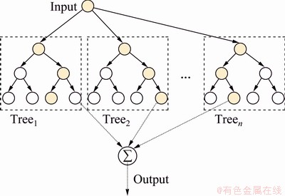
Fig. 11 Example of RF

5.3 Artificial neural networks

Artificial neural networks (ANN) mimic the working principle of neurons in the human brain and perform classification and prediction [31]. The smallest unit, called a neuron, produces an output such as Eq. (5), depends on the inputs, weights and activation function. The example of a neuron structure is shown in Fig. 12.

                       (5)

where o_i is the output results, n is the input size, w_i,j is the weight coefficient, and x_i,j is the input data.

In Eq. (5), input data x is weighted by weight w. Then, an activation function is applied to pushing linear sum to a non-linear space.

Fig. 12 Neuron structure for ANN model

The proposed ANN model with two hidden layers is shown in Fig. 13. There are 3 types of layers which are called as input, hidden and output. In the input layer, the number of neurons is determined by the number of feature vectors (for this study they are applied load, sliding distance and sliding speed). Numbers of hidden layers and neurons can be determined arbitrarily. Finally, the output layer (for this study it is wear volume loss) shows the estimated result according to computations by values from hidden layers. During training, the error between actual and predicted values is calculated and weights among neurons are updated using back propagation (BP) algorithm. This process continues until termination criterion is met or ANN has converged enough [32,33].

Fig. 13 Proposed ANN model

In order to compute error, root mean square error (RMSE) is used. It is calculated as follows (Eq. (6)):

                (6)

where e_i is the actual value, and p_i is the predicted value.

                    (7)

where  is the mean of the actual values and R² is the correction coefficient which represents the accuracy of the method, here, it is a commonly used performance measurement for machine learning methods. The desired result in machine learning methods is to produce a model with high R² and low RMSE values.

6 Experimental results of machine learning models

In this study, three machine learning algorithms (SVR, RF and ANN) were applied to estimating the wear volume loss of the AZ91 alloy. The experimentally collected data set was separated into training and test as 85% and 15%, respectively. Applied load, sliding distance and sliding speed were determined as input feature variables and the output was wear volume loss. RBF kernel function was employed for SVR method. In ANN model, the numbers of neurons located in hidden layers 1 and 2 were determined as 8 and 2, respectively (Fig. 13). Moreover, hyperbolic tangent was used as an activation function and the Quasi-Newton was used as a backpropagation algorithm. The results of the applied machine learning methods for training data can be seen in Fig. 14. According to the results, the highest accuracy (R²) for the training set was obtained by ANN. In addition, it was observed that RF is very competitive with ANN. Since the relationship between the data obtained from laboratory-based experimental results cannot be accurately estimated by hyperplanes, the accuracy of SVR decreased. When the incorrect results were analyzed, it was seen that the error increased especially in high wear volume loss values for ANN and SVR. This is because they produce more deviations for higher wear volume loss values.

Fig. 14 Comparison of experimental and predicted values for training data

The experimental and predicted results for test data are given in Table 4. Figure 15 shows the comparison of the results of the models with experimental ones for test data set. It was observed that the results obtained in the test set were similar to those in the training set. SVR achieved the lowest accuracy and ANN competed with RF. It was also noticed that ANN was more stable for both high and low output values. According to these results, it could be seen that the models did not over-fit training data (memorization of input data) and were able to learn the relationship between inputs and outputs.

Table 4 Comparison of experimental results and predicted results obtained with different models for test data set

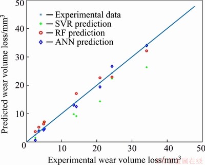
Fig. 15 Comparison of experimental and predicted values for test data

Furthermore, the effect of regularization constant (C) on R² for SVR was investigated (Fig. 16(a)). The model was tested with different C values from 0 to 10 with a step size of 0.1 (for plotting it is normalized to a range of 0-100) and had the highest accuracy when C was 1.5 (when inputs and training success are considered). As can be seen from Fig. 16(a), when C value was increased too much, even if the model achieved high accuracies for training set, it was observed that low accuracies were obtained in the test set because of over-fitting.

The effect of the number of estimators for RF was examined by testing from 0 to 1000 (Fig. 16(b)). The highest accuracies for both training and test sets were observed when the number of estimators was 40 and above. Therefore, considering the performance, it was seen that the most reasonable number of estimators was 40.

Fig. 16 Effect of SVR and RF parameters on R²

Table 5 presents the accuracies of the three methods. Although ANN and RF had almost the same accuracies for the test phase, SVR was far behind. Also, ANN had the higher accuracy than RF for the training stage.

Table 5 Comparison of accuracies of three methods

7 Conclusions

(1) The wear volume loss increased with increasing load for all sliding distances and some sliding speeds.

(2) The AFC values significantly changed depending on different sliding speeds, sliding distances and applied loads.

(3) At a load of 10 N, abrasive wear is the dominant mechanism under conditions of sliding distances of 250 and 1000 m and a sliding speed of 160 mm/s. However, oxidative wear emerges at a load of 10 N, a sliding speed of 220 mm/s and a sliding distance of 1000 m. Delamination is generally observed at a load of 50 N.

(4) ANOVA results show that the sliding distance is the most effective parameter for wear in AZ91 alloy.

(5) ANN can be used to estimate the wear volume loss of the AZ91 alloy with the highest accuracy (0.9845). In this way, high reliability estimation can be made for wear volume loss before performing experiments.

References

[1] SHANTHI M, LIM C Y H, LU L. Effects of grain size on the wear of recycled AZ91 Mg [J]. Tribology International, 2007, 40: 335-338.

[2] AYDIN F, TURAN M E. The effect of boron nitride on tribological behavior of Mg matrix composite at room and elevated temperatures [J]. Journal of Tribology, 2020, 142: 1-7.

[3] SONG J, SHE J, CHEN D, PAN F. Latest research advances on magnesium and magnesium alloys worldwide [J]. Journal of Magnesium and Alloys, 2020, 8: 1-41.

[4] AUNG N N, ZHOU W, LIM E N. Wear behaviour of AZ91D alloy at low sliding speeds [J]. Wear, 2008, 265: 780-786.

[5] TALTAVULL C, TORRES B, LOPEZ A J, RAMS J. Dry sliding wear behavior of AM60B magnesium alloy [J]. Wear, 2013, 301: 615-625.

[6] ZAFARI A, GHASEMI H M, MAHMUDI R. Tribological behavior of AZ91D magnesium alloy at elevated temperatures [J]. Wear, 2012, 292-293: 33-40.

[7] CHEN H, ALPAS A T. Sliding wear map for the magnesium alloy Mg-9Al-0.9 Zn (AZ91) [J]. Wear, 2000, 246: 106-116.

[8] WANG S Q, YANG Z R, ZHAO Y T, WEI M X. Sliding wear characteristics of AZ91D alloy at ambient temperatures of 25-200 °C [J]. Tribology Letters, 2010, 38: 39-45.

[9] VIGNESH R V, PADMANABAN R. Forecasting tribological properties of wrought AZ91D magnesium alloy using soft computing model [J]. Russian Journal of Non-Ferrous Metals, 2018, 59: 135-141.

[10] HIMANEN L, JAGER M O J, MOROOKA E V, CANOVA F F, RANAWAT Y S, GAO D Z, RINKE P, FOSTER A S. Dscribe: Library of descriptors for machine learning in materials science [J]. Computer Physics Communications, 2020, 247: 1-13.

[11] CARUANA R, NICULESCU-MIZIL A. An empirical comparison of supervised learning algorithms [C]// Proceedings of the 23rd International Conference on Machine Learning. Pittsburgh, 2006: 161-168.

[12] KAVIMANI V, PRAKASH K S. Tribological behaviour predictions of r-GO reinforced Mg composite using ANN coupled Taguchi approach [J]. Journal of Physics and Chemistry of Solids, 2017, 110: 409-419.

[13] UPASE R, AMBHORE N. Experimental investigation of tool wear using vibration signals: An ANN approach [J]. Materials Today: Proceedings, 2020, 24: 1365-1375.

[14] HUSSIEN R M, AL-SHAMMARI M A. Prediction of physical and mechanical properties of aluminum metal matrix composite using artificial neural networks [J]. Journal of Mechanical Engineering Research and Developments, 2020, 43: 409-416.

[15] GOODFELLOW I, BENGIO Y, COURVILLE A. Deep learning [M]. Massachusetts: MIT Press, 2016.

[16] PILANIA G, WANG C, JIANG X, RAJASEKARAN S, RAMPRASADR. Accelerating materials property predictions using machine learning [J]. Scientific Reports, 2013, 3: 1-6.

[17] RAMPRASAD R, BATRA R, PILANIA G, MANNODI- KANAKKITHODI A, KIM C. Machine learning in materials informatics: Recent applications and prospects [J]. npj Computational Materials, 2017, 3: 1-13.

[18] PARK S S, PARK Y S, KIM N J. Microstructure and properties of strip cast AZ91 Mg alloy [J]. Metals and Materials International, 2002, 8: 551-554.

[19] KABIRIAN F, MAHMUDI R. Impression creep behavior of a cast AZ91 magnesium alloy [J]. Metallurgical and Materials Transactions A, 2009, 40: 116-127.

[20] GARCIA-RODRIGUEZ S, TORRES B, MAROTO A. Dry sliding wear behavior of globular AZ91 magnesium alloy and AZ91/SiC_p composites [J]. Wear, 2017, 390-391: 1-10.

[21] ABBAS A, HUANG S J, BALLOKOVA B, SULLEIOVA K. Tribological effects of carbon nanotubes on magnesium alloy AZ31 and analyzing aging effects on CNTs/AZ31 composites fabricated by stir casting process [J]. Tribology International, 2020, 142: 105982.

[22] AYDIN F, SUN Y, TURAN M E. Influence of TiC content on mechanical, wear and corrosion properties of hot-pressed AZ91/TiC composites [J]. Journal of Composite Materials, 2020, 54: 141-152.

[23] AYDIN F, SUN Y, TURAN M E. The effect of TiB₂ content on wear and mechanical behavior of AZ91 magnesium matrix composites produced by powder metallurgy [J]. Powder Metallurgy and Metal Ceramics, 2019, 57: 564-572.

[24] NGUYEN Q B, SIM Y H M, GUPTA M, LIM C Y H. Tribology characteristics of magnesium alloy AZ31B and its composites [J]. Tribology International, 2015, 82: 464-471.

[25] VAPNIK V. Pattern recognition using generalized portrait method [J]. Automation and Remote Control, 1963, 24: 774-780.

[26] VAPNIK V. A note one class of perceptrons [J]. Automation and Remote Control, 1964, 25: 103-109.

[27] VAPNIK V, GOLOWICH S E, SMOLA A J. Support vector method for function approximation, regression estimation and signal processing [C]//Advances in Neural Information Processing Systems. Denver: MIT Press, 1997: 281-287.

[28] SCHLKOPF B, SMOLA A J, BACH F. Learning with kernels: Support vector machines, regularization, optimization, and beyond [M]. Massachusetts: MIT Press, 2018.

[29] RASI R E, NAMAKAVARANI O M. Organizational agility considering enablers and capabilities of agility with RBF neural network approach and multiple regressions [J]. International Journal of Information Technology, 2020: 1-20.

[30] BREIMAN L. Random forests [J]. Machine Learning, 2001, 45: 5-32.

[31] JACEK M Z. Introduction to artificial neural systems [M]. Minnesota: West Publishing Company, 1992.

[32] GLOROT X, BENGIO Y. Understanding the difficulty of training deep feedforward neural networks [C]//Proceedings of the Thirteenth International Conference on Artificial Intelligence and Statistics. 2010: 249-256.

[33] GARDNER M W, DORLING S R. Artificial neural networks (the multilayer perceptron)—A review of applications in the atmospheric sciences [J]. Atmospheric Environment, 1998, 32: 2627-2636.

机器学习法预测AZ91合金在干滑动摩擦条件下的磨损性能

Fatih AYDIN¹, Rafet DURGUT²

1. Department of Metallurgical and Materials Engineering, Karabuk University, Karabuk, Turkey;

2. Department of Computer Engineering, Karabuk University, Karabuk, Turkey

摘  要：研究在不同载荷(10~50 N)、滑动速度(160~220 mm/s)及滑动距离(250~1000 m)条件下AZ91合金的磨损行为。结果表明，在一定的滑动距离和滑动速度下，磨损体积损失随负载的增加而增加。当滑动速度为220 mm/s和滑动距离为1000 m时，载荷10、20、30、40及50 N下合金的体积损失分别为15.0、19.0、24.3、33.9及37.4 mm³。磨损表面显示，载荷为10 N时磨损表面存在磨损和氧化现象，载荷为50 N时发生分层现象。ANOVA结果显示，载荷、滑动距离和滑动速度的贡献率分别为12.99%、83.04%及3.97%。采用人工神经网络(ANN)、支持向量回归(SVR)和随机森林(RF)对AZ91合金的体积损失进行预测。SVR、RF及ANN的相关系数(R²)分别为0.9245、0.980及0.9845。因此，ANN模型能较好地预测AZ91合金的耐磨性能。

关键词：AZ91合金；磨损性能；人工神经网络；支持向量回归；随机森林方法

(Edited by Wei-ping CHEN)

Corresponding author: Fatih AYDIN; E-mail: fatih.aydin@karabuk.edu.tr

DOI: 10.1016/S1003-6326(20)65482-6

1003-6326/ 2021 The Nonferrous Metals Society of China. Published by Elsevier B.V. & Science Press