J. Cent. South Univ. (2018) 25: 2245-2257

DOI: https://doi.org/10.1007/s11771-018-3910-9

Anomaly detection in traffic surveillance with sparse topic model

XIA Li-min(夏利民), HU Xiang-jie(胡湘杰), WANG Jun(王军)

School of Information Science and Engineering, Central South University, Changsha 410083, China

Central South University Press and Springer-Verlag GmbH Germany, part of Springer Nature 2018

Abstract: Most research on anomaly detection has focused on event that is different from its spatial-temporal neighboring events. It is still a significant challenge to detect anomalies that involve multiple normal events interacting in an unusual pattern. In this work, a novel unsupervised method based on sparse topic model was proposed to capture motion patterns and detect anomalies in traffic surveillance. scale-invariant feature transform (SIFT) flow was used to improve the dense trajectory in order to extract interest points and the corresponding descriptors with less interference. For the purpose of strengthening the relationship of interest points on the same trajectory, the fisher kernel method was applied to obtain the representation of trajectory which was quantized into visual word. Then the sparse topic model was proposed to explore the latent motion patterns and achieve a sparse representation for the video scene. Finally, two anomaly detection algorithms were compared based on video clip detection and visual word analysis respectively. Experiments were conducted on QMUL Junction dataset and AVSS dataset. The results demonstrated the superior efficiency of the proposed method.

Key words: motion pattern; sparse topic model; SIFT flow; dense trajectory; fisher kernel

Cite this article as: XIA Li-min, HU Xiang-jie, WANG Jun. Anomaly detection in traffic surveillance with sparse topic model [J]. Journal of Central South University, 2018, 25(9): 2245–2257. DOI: https://doi.org/10.1007/s11771-018- 3910-9.

1 Introduction

There is an urgent need for fully automated and unsupervised anomaly detection system with the rapid growth of monitors in public area. This is particularly true for traffic surveillance. High efficiency video anomaly detection system is of great significance and has become one of the most popular researches. Due to the complexity of the video scene and the diversity of events, video anomaly detection is still a challenging problem [1].

In general, video anomaly detection method can be classified into two categories: individual anomaly detection and interactive anomaly detection. Individual anomaly is defined as an event that is different from other normal events. It is usually distinguished by the difference of the object features [2]. Interactive anomaly usually involves multiple events which occur simultaneously and interact in an unusual manner [3]. Most of the current methods have focused on individual anomalies such as objects with unusual appearance, speed or motion trajectories [4–7]. REN et al [4] used the temporal neighborhoods of video features to generate a local space and applied K spectral clustering to obtain the normal space. Then the local space and normal space were compared to find the abnormal features when the difference was large. XIA et al [5] decomposed human behaviors into multiple sub-behaviors with a visual attention model and used the incremental case-based reasoning approach to distinguish the abnormal behaviors. ROSHTKHARI et al [6] built a spatial- temporal volume for each interest point which was the center of the volume, and used the fuzzy mean clustering method to cluster the features. Abnormal events were detected by calculating the distance between the events and the normal spatial and temporal contexts. BISWAS et al [7] divided the video scene into several blocks and computed the dictionary for each block. Then the local dictionary was enhanced by the similarity of normal behaviors in the adjacent blocks and anomaly was detected using the sparse reconstruction error.

Interactive anomaly is more difficult to recognize than the individual anomaly, since it should be determined by the relationship of multiple events while each event may be normal in the separate analysis. In order to deal with the interactive anomaly, the group interaction information has been utilized in many methods. CUI et al [8] proposed an interaction energy potential function to describe the current state of the object and discovered the relationship between the state and its actions. SVM was applied to detecting abnormal behaviors in group activities. BERA et al [9] proposed an algorithm for interpersonal interaction learning which was able to track the object and analyze the interaction behavior of the crowd in real-time. MEHRAN et al [10] applied the bag of words method to classify the frames into normal and abnormal, and employed the social force model to evaluate the interaction forces which were used to find the location of anomalies in anomalous frames.

However, these approaches are aimed at human activities and may not be suitable for traffic scenes [11]. Therefore, many methods model the events that occur simultaneously to describe the video scene. CHENG et al [12] applied a hierarchical framework to describe the individual and interactive feature of video, and then used the Gaussian process regression (GPR) model to explore the mathematical relationships of the adjacent spatial-temporal interest points and detect anomalies. MO et al [13] presented a joint sparsity model (JSM) to obtain the over-complete dictionary of trajectories and used it to detect the interactive abnormal events that involve multiple objects. These methods adopt the data trained from the training samples to reconstruct the test videos, and anomalies are determined with the reconstruction cost. Although it can usually achieve a good detection performance, there is a lack of semantic description of the video scene. In the semantic analysis of video, the probabilistic topic models have achieved great success [14]. Topic models can obtain latent motion patterns which represent the common distributions of the scene and detect anomalies with likelihood values. EMONET et al [15] and VARADARAJAN et al [16] mined activity motifs in video scenes with topic models such as Bayesian network, which was efficient in trajectory representation and prediction. YOO et al [17] applied a two-layered probabilistic model to find major patterns in a crowd scene and predicted the path of targets. FU et al [18] proposed a sparse topical coding (STC) method to discover the latent motion patterns of video and viewed the video scene as a combination of these patterns. JEONG et al [19] proposed a topic model based method to check the violation of traffic rule. PATHAK et al [20] used the topic model such as PLSA for the video scene analysis, and abnormal events were detected by constructing a topic space. However, in general, the abnormal events in a video clip only occur in a small spatial and temporal region, so the difference of likelihood between normal video clips and abnormal video clips is not significant, which limits the efficiency of the anomaly detection.

To address these problems, the sparse topic model has been put forward. It is derived from the probabilistic topic model, initialized by the probability density function and finally expressed in a non-probabilistic form. This model can not only capture the motion patterns, but also use them to encode the visual words and achieve a sparse representation for the video scene. So anomaly can be detected with individual word analysis to improve the accuracy.

The main contributions of this paper include:1) SIFT flow method is applied to obtaining dense trajectories instead of optical flow, which has been proved to be more robust to get the motion information; 2) To enhance the spatial and temporal relations of interest points, the fisher kernel method is employed to describe each trajectory and the video is treated as a document consisting of visual words which are generated by trajectories; 3) The sparse topic model is constructed to discover the motion patterns and detect anomalies.

2 Improved dense trajectory with SIFT flow

In order to detect the abnormal events in a video, we first need to extract the interest points and obtain the motion features to describe the video scene. The motion features should be rich enough to be able to capture any possible event in a video. In this work, the dense trajectory method is adopted to extract feature points, since it has been shown to be efficient for video representation [21]. Meanwhile, because there are always lots of interference in traffic videos such as illumination changes, SIFT flow is used to track the trajectory to improve the performance.

2.1 SIFT flow method

SIFT flow can be seen as derived from the optical flow, which uses the SIFT descriptor to discover the relationship of corresponding pixels between two adjacent images and establishes motion flow vector according to the similar algorithm to optical flow. It is more robust to get the motion information of the pixels from two adjacent frames [20].

For every pixel in a frame, we divide its neighborhood into 4×4 cell array, quantize the orientation into 8 bins in each cell, and obtain a 128 (4×4×8) dimensional vector as the SIFT descriptor. After getting the SIFT feature vectors of all pixels, we can get a corresponding abstract image called SIFT image. The pixel value in SIFT image refers to the SIFT descriptor of the corresponding pixel in the original image, so it contains rich local information and has high spatial resolution.

Review the generative process of optical flow which is discovered based on the correlation of the pixel intensity in two adjacent frames. This process is also applicable to SIFT images. It can be utilized to find the point-to-point correspondences between adjacent SIFT images and determines a flow vector similar to optical flow which is called SIFT flow. Assuming a pixel point P in the image, its corresponding motion flow vector is recorded as ω(P)=(u(P), v(P)). We can get the following objective energy function:

       (a)

                (b)

       (c)    ₍₁₎

where s₁(·) and s₂(·) denote the corresponding pixel values of two adjacent SIFT images which are equivalent to the SIFT descriptors of original images; t₁ and t₂ are thresholds for removing outliers and flow discontinuities; Q is a point in the neighbor of P. The energy function of SIFT flow consists of three terms: the data term, the small displacement term and the smoothness term. The data term (a) aims to match the corresponding points between adjacent images by computing the difference of their SIFT descriptors; the small displacement term (b) is used to limit the size of the flow vector; the smoothness term (c) makes sure the smoothness of local regions by minimizing the difference between the pixel and its neighbors. It can be optimized with the similar method used in the optimization of optical flow [22].

2.2 Trajectory extraction method

Each frame is divided into grids with a size of W×W pixels. Interest points are extracted in these spatial grids and they are tracked separately in multiple spatial scales. The spatial scales are at most 8 which are determined by the resolution of video and they are increased at a rate ofto ensure that sufficient interest points are obtained. It has been proved that when W=5, the trajectories are dense enough to achieve a good representation for the video. Each interest point P_t=(x_t, y_t) in frame t is tracked through the SIFT flow ω_t=(u_t, v_t) to find the corresponding points in the next frame as:

      (2)

wheredenotes the rounded position of (x_t, y_t) and F is the nuclear of median filtering with a size of 3×3 pixels.

The tracking lasts for L frames and the trajectory is generated after getting the relevant interest points in the consecutive frames. When there is no point found in the spatial grid, another new interest point will be sampled and tracked to make sure the density of trajectories. In traffic surveillance, what we are most concerned about is the position and motion orientation of objects. Therefore, the feature vector of point P_t is denoted by (x_t, y_t, θ), where θ is the angle of flow vector and it is quantized into eight directions.

3 Trajectory and video representation

After obtaining the dense trajectories and the feature vector of each interest point, we will use these information to describe the trajectory and video.

3.1 Trajectory representation with fisher kernel

Most methods directly describe the video with complex feature vectors of interest points and ignore the information of trajectory which is only represented by the trajectory shape descriptor calculated by the coordinate offset of interest points in two adjacent frames. However, in this work, the video scene is regarded as composed of lots of trajectories and we consider that the representation of trajectory is of great significance.

To address this problem, we adopt a method based on fisher kernel to represent the trajectory, that is, using a probability density function to approximate the trajectory. It is based on adopting the parameter generation model to fit the descriptors, and then using the log-likelihood derivatives of the model parameters to be the representation. Let Z={z_t, t=1, …, L} denote the set of interests points on the trajectory, where z_t is the feature descriptor of each interest point. In the fisher kernel framework [23], these features are considered to conform to a certain distribution and be independent of each other, and the Gaussian mixture model (GMM) can be utilized to model the generation process of Z with a probabilistic distribution function p and the parameter set where ω_i, μ_i, and Σ_i represent the weight, mean vector and covariance matrix of Gaussian i respectively and I denotes the number of Gaussian. The GMM is learned in the training set using maximum likelihood (ML) estimation [24]. It is supposed to be able to describe all the information of trajectories.

LetWith the independence assumption, it can also be denoted as:

                    (3)

The probability of z_t which is generated by the GMM is denoted as:

                    (4)

where the sum of the weights is equal to 1, and the probabilistic distribution function p_i is:

         (5)

where β denotes the dimension of the feature vectors which is 3 here. Then let γ_t(i) denote the soft assignment of t-th descriptor z_t to the i-th Gaussian:

                      (6)

The covariance matrices are assumed to be diagonal for two reasons: 1) any distribution can be approximated with arbitrary precision by a weighted sum of Gaussian with diagonal covariances and 2) the calculation of diagonal covariances is much simpler than the full

covariances. It is denoted by Let ζ_μ,i and ζ_σ,i denote the gradient vector of the mean μ_i and the standard deviation σ_i of Gaussian i respectively.

                 (7)

           (8)

The final feature vector of trajectory is then represented by the concatenation of these two vectors for i=1, …, I, with a size of 2×I×β. Figure 1 shows the generation process of trajectory descriptor.

3.2 Video representation

Given an input video under a traffic surveillance, temporally divide them into equal-length clips without overlapping. We use the trajectory representation to generate visual words and each video clip is represented with these visual words.

To get the visual words and vocabulary, the interest points are tracked for each video clip and trajectories are represented as feature vectors as described above. The K-means clustering method is applied to cluster all these trajectories and obtain N cluster centers. Each cluster center corresponds to a visual word. Therefore, a vocabulary can be denoted as V={v₁, v₂, …, v_N}, where represents a visual word of the video.

Figure 1 Generation of trajectory descriptor

After getting the vocabulary, the video clip can be seen as a document composed of visual words. For a video document d, we classify the trajectories to the cluster centers with minimum Euclidean distance and count the number of occurrence for every visual word.

                   (9)

wheredenotes the number of occurrence of word v_n in this document.

4 Construction of sparse topic model

With the knowledge of topic model, assume that there are K topics in the video document, each topic is made up of a variety of trajectories and can be regarded as a distribution over the vocabulary. We combine the topics to form a matrix which is called topic dictionary. Each row D_k is a topic base equivalent to a motion pattern. The model projects d into a semantic space spanned by the dictionary and obtain the word code vector for each individual word in document d. I_d denotes the set of words whose counts are not zero in document d. For the word , its corresponding code is equal to zero. Thus, the whole document can be represented by the code set and the dictionary D.

4.1 Probabilistic generative process

Each visual word in documents belongs to some semantic topics which correspond to the motion patterns in video flow. Therefore, each document can be viewed as composed of different topics. The key of the sparse topic model is to use the topic bases to discover sparse representation for large scale video data. The generative process of the model can be summarized as follow. Take M clips to form the training set S. For each topic

1. Sample the topic base D_k based on a uniform prior distribution p(D_k).

2. For each document dS:

1) Sample the word code vector α_d,k from a prior distribution p(α_d,k).

2) For each visual word nI_d:

Sample the word count w_d,n from a conditional distribution

In this process, it is assumed that word counts are independent of each other and each word has independent relationship with different topics. The word counts can be reconstructed by the linear combination of topic dictionary D and the code set and then the document can be interpreted by the model. For a document d, a joint probability distribution can be defined as:

    (10)

In order to get sparse representation for each document, it is necessary to make sure that only a few topics contribute to the document codes while the word codes in other topics are equal to zero. So we consider that word codes are in group structure. This could be achieved by grouping the word codes under the same topic together and sample the groups of variable from a multivariate Laplace distribution [25] (see Eq. (11)). The multivariate Laplace prior over each group of coefficients transforms the group-lasso constraints into a MAP-solution in the logarithmic space.

 (11)

For every word that occurs in the document, the number of the occurrence is equal to the summation of the word counts over different topics. Suppose the word counts conform to the Poisson distribution:

 (12)

The reason why we choose the Poisson distribution with the parameter α_nkD_kn is that: 1) it is convenient to constrain the non-negative feasible domains of word codes with good interpretation; 2) the mathematical properties of Poisson distribution, such as additive property, match the nature of word counts.

The joint probability distribution function of the model can be determined through the above formulas. Because p(α, w, D) is less than 1, in order to obtain the maximum value of the probability distribution, define the objective function as follow:

                    (13)

The frequencies of different topics are not the same in video scenes, which means that the importance of each topic is different. Due to this characteristic, we add an 1-norm constraint term for the column vector of D to the objective function, which can also improve the sparsity of dictionary. Then the final optimization function is as follow:

        (14)

where the hyper-parameters λ₁ and λ₂ are non- negative and can be selected via cross-validation. The first part of the objective function is a loss function, which is equivalent to the KL divergence between the word count and its reconstruction. When it gets the minimum value, it means that the reconstructed value is the closest to the real one. The second part is a group lasso, which is used to induce the sparsity of the document codes. The third part denotes the number of the zero value in the dictionary. Since each topic is only related to a limited number of visual words, adding this constraint term can force the model to learn motion topics with less correlations.

Although the sparse topic model is derived from the probabilistic model, it is ultimately expressed in a non-probabilistic form. By optimizing the objective function, we can not only obtain motion patterns with good independence but also achieve the sparse representation for the documents. By using this model to reconstruct the test documents, the abnormal events can be detected with subsequent analysis.

4.2 Model optimization

Because there are two variables in the objective function, a similar optimization strategy is adopted as proposed in Ref. [17], that is, optimizing the function with only one variable while the other is assumed to be fixed. Alternatively perform the optimization over α and D until the convergence of the objective function. The process of optimization over α is called sparse coding, while the process of optimization over D is called dictionary updating.

4.2.1 Sparse coding

In the sparse coding process, since the documents are independent of each other, we can solve the following problem alternately for each document:

                    (15)

The above function is recorded as g(α_d) and it is convex over α_d. So the coordinate decent method can be used for this optimization by solving the problem for each element alternatively. The proof process is described below. First deriving the function:

       (16)

where ε is a small enough positive number which is used to avoid the denominator equaling zero. Then taking the second derivative

 (17)

Obviously, the value of the above formula is always positive, so formula (15) is strictly convex for each α_d,nk and its minimum value will be obtained at the extreme point. By setting formula (16) equal to zero, it transforms to a quadratic equation. The optimal solution of the objective function can be obtained by solving this equation.

LetSince the value of word codes should be no less than zero, the final solution is

4.2.2 Dictionary updating

In the dictionary updating process, the problem transforms to minimize the following formula ξ(D):

                         (18)

Since the elements of dictionary are all non- negative, the constraint term can be represented as:

                  (19)

Here we adopt a similar solution to the sparse coding process described above. That is, solving the problem for each element of dictionary alternatively. Taking the derivative on D_kn.

         (20)

Obviously, Eq. (20) has a similar structure to formula (16), and the objective function is also strictly convex. Hence, the minimum value will be obtained when formula (20) equals zero. Let the optimal valuethe solution is .

From the above formula, it can be seen that D_kn is inversely proportional to the parameter λ₂. When the parameter gets larger, the value of elements will become smaller, so there is likely to be more atoms coming to zero in D. These two processes are repeated until the result of formula (14) converges to get the final optimization result.

5 Anomaly detection using sparse topic model

Abnormal events have various definition in different methods. Most methods treat events that have not appeared or cannot be accurately described by models as anomalies. However, we define it as the event that deviates from the normal motion patterns, in other words, an event happened at an unusual location or at an unusual time. The judgment of abnormality is closely related to the dynamic scenes.

5.1 Clip detection

Through the training samples, we can get the dictionary of the model and then use it to represent the test samples, so as to get the corresponding document codes. Several algorithms based on the resulting codes are proposed here to detect anomalies in video test samples. In the process of model construction, a number of topics are obtained, which correspond to the motion patterns. Each dynamic scene in the video can be viewed as a combination of several motion patterns. The video clips containing anomaly are called abnormal clips. To detect the abnormal clips, the reconstruction cost is defined as:

 (21)

Obviously, a clip with a high value is more likely to contain anomalies. Since the simulations show that the results of abnormality detection by using L_d with and without the sparsity term of code vectors are the same, and in order to demonstrate the reconstruction process better, the reconstruction vector is set to be The reconstruction accuracy is defined as:

                      (22)

where (w_d, R_d) denotes the inner product of the two vectors. When the reconstruction accuracy gets smaller, it means the deviation between the test clip and the normal motion patterns gets larger, and they are more likely to be abnormalities in the document. A threshold can be obtained through experiments which can be used to distinguish between normal clip and abnormal clip. When the reconstruction accuracy is less than the threshold, it is recorded as an abnormal clip.

5.2 Word evaluation

The value of reconstruction accuracy is sensitive to the quantity of anomalies. Since each document contains a large amount of information and abnormal event usually occurs in a small spatial-temporal domain, there is not much difference between normal and abnormal clips. Hence, we present an approach for individual evaluation of visual words in test video clips. The details of the algorithm are shown below:

1) With the learned word codes we can obtain the proportion of each topic in document. The expected admixture proportion of document d on k-th topic can be calculated by

                     (23)

Then each clip d_i is represented as a distribution over topic space as

2) For a test clip, first project it into the topic space and get the corresponding vector. In order to describe the similarity between two clips, the distance between the clips d_i and d_j is calculated by

             (24)

3) Find the m nearest training samples in the topic space as described above. Let H_i denote the histogram of word counts in clip d_i. Then the histograms of all its m nearest training clips are counted into a histogram H₀.

4) Then explore every word v_n that appears in the test clip at least once. If the count of v_n in histogram H₀ is greater than a certain threshold, it will be recorded as a normal word.

5) If v_n does not conform to step 4, then record it as an anomalous word. The test clip will be called abnormal if the number of anomalous words in it reaches a specific value. Because each visual word is generated by the trajectory feature, what we actually obtain is the information of anomalous trajectories.

6 Experiments

In order to evaluate the performance of our proposed method, experiments were executed on two complex public traffic datasets, namely QMUL Junction dataset and AVSS dataset. The proposed approach was applied to detecting abnormal events in these two datasets, and then the detection results were compared with other state-of-the-art methods to verify the effectiveness of our method.

6.1 QMUL Junction dataset

This dataset is composed of a surveillance video located at a busy traffic junction. The video is captured at 25 frames per second. It is about 52 min long and contains 78000 frames with a frame size of 360×288 pixels. The content of the video is quite complex. Its background consists of four roads, two sidewalks and many surrounding buildings. Each scene contains a large number of vehicles, bicycles and pedestrians with strong light changes. Meanwhile, there are various activities, including vehicles straight driving, turning, waiting for the red lights and pedestrians crossing the road.Figure 2 shows some typical simple motion patterns of the video. Each motion pattern is actually made up of simultaneous trajectories in video scene. So it includes not only simple patterns but also composite patterns combined by those simple ones, such as a pattern consisting of vehicle straight driving pattern and turning pattern. There are two cases of abnormal events. The first is event deviating from the normal motion pattern, such as vehicle retrograde; the other is the case that two conflict topics occur simultaneously. For example, as shown in Figures 2(b) and (c), when the vechile is traveling with pedestrians passing, it means an abnormal event happens. Figure 5 shows some abnormal examples of the test clips.

The video was divided into non-overlapping fragments with a length of 4 s. The video clips containing abnormal activities were first separated out. 75% of the remaining video clips were then selected for the model training to get the topic dictionary, and the other clips were used for anomaly detection.

1) Selection of parameters

To learn the trajectory descriptors and quantify the video to visual document, we learned the GMM with I=10 components. For the parameters λ₁ and λ₂, they were supposed to take appropriate values. Too small parameters would lead to a low sparsity model, while a model with highly sparse codes and dictionary might miss some useful information. We experimentally found the best result with the parameters λ₁=0.4 and λ₂=200. For the number of topics, without a prior knowledge, different values were used in the experiment to find out the best detection result as shown in Figure 3.

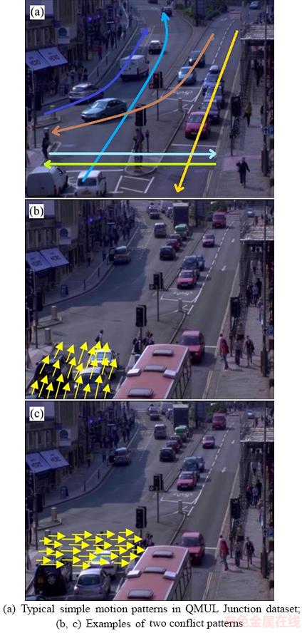
Figure 2 Images of events:

In order to fully demonstrate the detection efficiency of the method, the F1-measure which is defined as the harmonic mean of the precision and the recall is employed to show the performance of our method. Figure 3 takes the topic number as the abscissa axis and the maximum F1 value is achieved by the two anomaly detection algorithms as the ordinate axis. From Figure 3, we can know that when K=20, the model can achieve the highest detection accuracy.

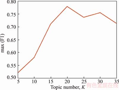
Figure 3 Detection performance with different topic number

2) Comparison of representation methods

The SIFT flow-based dense trajectory was compared with the optical flow-based dense trajectory [21] to verify the effectiveness of the proposed SIFT flow method in video anomaly detection. We conducted experiments with different trajectory representation methods too. Table 1 shows the detection results using different trajectory extraction and representation methods. From Table 1, we can observe that the proposed improved dense trajectory method is more distinguished in video anomaly detection; the algorithm of abnormal word detection can achieve a higher accuracy than the clip detection algorithm.

Table 1 Comparison of different trajectory extraction and representation methods using F1-measure

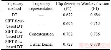
Trajectory descriptor generated by the fisher kernel performs better than the concatenation. One of the reasons is that the fisher kernel based trajectory feature extraction method does not require a fixed number of interesting points for each trajectory, so it can capture more short-term and long-term trajectories and increase the density of the trajectories. In addition, the location and shape information of the trajectory are modeled as a whole, which enhances its structure feature and achieves higher discrimination, thus a more complete codebook can be obtained.

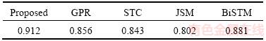
3) Comparison of different detection methods

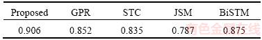
We compared the results detected by word evaluation algorithm with some other state-of-the- art methods such as GPR [12], JSM [13], STC [18] and BiSTM [26]. Figure 4 shows the ROC curves of these methods on QMUL Junction dataset and Table 2 shows the corresponding AUC values.

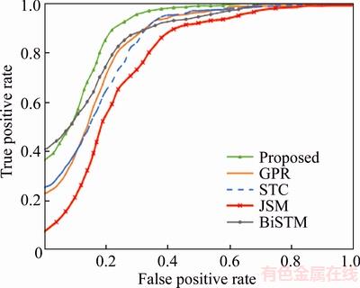
Figure 4 ROC curves on QMUL Junction dataset

Table 2 AUC values of different methods on QMUL dataset

6.2 AVSS dataset

The dataset was released as a part of the i-LIDS vehicle detection challenge in AVSS 2007. It consists of a video recorded by a suburban street surveillance camera. The main movements in the video include the left-lane vehicle going up, the right-lane vehicle going down, vehicle turning, pedestrian crossing the road and so on. In the video scene, in addition to the changes in light intensity, there is also instability caused by the camera shake. Hence, there are still great challenges in the analysis of the video. Figure 6 shows some typical abnormal examples of AVSS dataset. We tried the parameter settings in the previous dataset which also achieved a good performance in AVSS dataset. Hence, the same parameters were used here.

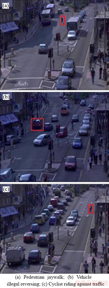
Figure 5 Typical examples of test samples in QMUL Junction dataset:

In order to show the performance of the proposed model in terms of capturing motion patterns and the sparsity of video representation, we have defined two measures called topic similarity (TS, S_t) and word sparsity (WS, S_w). WS is calculated based on the proportion of zero entries in word codes. TS is calculated based on average correlation between each two different topics:

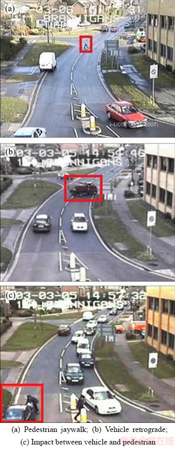
Figure 6 Typical examples of test samples in AVSS dataset:

             (25)

We compared our method with some typical topic models as shown in Table 3. It can be observed that the topic similarity of our method is significantly lower than the others, which indicates that the correlation between each motion pattern is low and the independence is strong. The WS values on the two datasets are 0.953 and 0.962, respectively. STC is similar to the proposed model which also has good sparsity. However, the biggest difference is that we ignore the document codes in the modeling process which makes the STC require more data in learning. We regard it as a derivative of word codes, so the model focuses more on topic bases and word codes, making the training process more simple and achieving higher sparsity.

The ROC curves of different methods on AVSS dataset are shown in Figure 6 and the AUC performance is summarized in Table 4.

Table 3 Topic similarity of different topic models

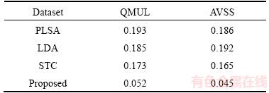
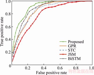
Figure 7 ROC curves on AVSS dataset

Table 4 AUC values of different methods on AVSS dataset

From Tables 2 and 4, it can be observed that compared with other state-of-the-art approaches, the proposed method can achieve a better performance in anomaly detection. JSM based method extracts the motion trajectory to analyze the traffic scenes but ignores the events happened in unusual manners. STC and GPR are two representative methods that can obtain individual and interactive information for video analysis and detect anomalies from global methods such as reconstruction cost and likelihood. BiSTM adds a layer of one-class SVM to STC and uses label information to achieve semi-supervised learning, which improves the efficiency of discriminating abnormal clips. However, the whole clip detection method still limits the detection accuracy. The proposed method uses the features of trajectories instead of interest points to generate visual words, which can greatly increase the amount of information in words. Each visual word is then evaluated individually through motion pattern analysis to improve the anomaly detection performance.

Typical probabilistic topic models focus on discovering the latent semantic of data, which can describe the video effectively, but lacks sufficient discrimination. The proposed sparse topic model can be inferred in a fully optimization manner, making it obtains the advantages of sparse representation model. The constraints are introduced to the topics and codes, which ensures the topics in a group structure and achieves efficient coding. The topic dictionary atoms that contribute little to the video scene modeling are effectively eliminated, so the discrimination and presentation ability of the entire model is enhanced.

The experiments are all conducted on a computer with 4 GB RAM and 3 GHz CPU. The average computation time is 1.7 s/frame for QMUL Junction dataset, and 1.4 s/frame for AVSS dataset.

7 Conclusions

1) A method for video anomaly detection based on sparse topic model is proposed. This method has obvious advantages in motion pattern discovery and abnormal event detection.

2) SIFT flow method is applied to improving dense trajectories, and the trajectory features are utilized to generate visual words, which can greatly increase the detection accuracy when the word is evaluated individually.

3) The proposed sparse topic model is actually a non-probabilistic topic model. It captures the groups of co-occurring trajectory features. This leads to dominant motion patterns which are further used to describe unseen video clips and detect anomalies.

4) Two datasets are used to test the proposed methods: QMUL Junction dataset and AVSS dataset. The experimental results demonstrate the feasibility and the effectiveness of our method.

References

[1] LEYVA R, SANCHEZ V, LI C. Video anomaly detection based on wake motion descriptors and perspective grids [C]// IEEE International Workshop on Information Forensics and Security. IEEE, 2015: 209–214.

[2] PICIARELLI C, FORESTI G L. Surveillance-oriented event detection in video streams [J]. IEEE Intelligent Systems, 2010, 26(3): 32–41.

[3] CONG Y, YUAN J, LIU J. Sparse reconstruction cost for abnormal event detection [C]// IEEE Conference on Computer Vision and Pattern Recognition. IEEE Computer Society, 2011: 3449–3456.

[4] REN H, MOESLUND T B. Abnormal event detection using local sparse representation [C]// IEEE International Conference on Advanced Video and Signal Based Surveillance. IEEE, 2014: 125–130.

[5] XIA Li-min, YANG Bao-juan, TU Hong-bin. Recognition of suspicious behavior using case-based reasoning [J]. Journal of Central South University, 2015, 22(1): 241–250.

[6] ROSHTKHARI M J, LEVINE M D. Online dominant and anomalous behavior detection in videos [C]// Computer Vision and Pattern Recognition. IEEE, 2013: 2611–2618.

[7] BISWAS S, BABU R V. Sparse representation based anomaly detection with enhanced local dictionaries [C]// IEEE International Conference on Image Processing. IEEE, 2015: 5532–5536.

[8] CUI X, LIU Q, GAO M, METAXAS D N. Abnormal detection using interaction energy potentials [C]// Computer Vision and Pattern Recognition. IEEE, 2011: 3161–3167.

[9] BERA A, KIM S, MANOCHA D. Realtime anomaly detection using trajectory-level crowd behavior learning [C]// IEEE Conference on Computer Vision and Pattern Recognition Workshops. IEEE Computer Society, 2016: 1289–1296.

[10] MEHRAN R, OYAMA A, SHAH M. Abnormal crowd behavior detection using social force model [C]// Conference on Computer Vision and Pattern Recognition, 2009. IEEE, 2009: 935–942.

[11] AHMADI P, TABANDEH M, GHOLAMPOUR I. Abnormal event detection and localisation in traffic videos based on group sparse topical coding [J]. Let Image Processing, 2015, 10(3): 235–246.

[12] CHENG K W, CHEN Y T, FANG W H. Gaussian process regression-based video anomaly detection and localization with hierarchical feature representation [J]. IEEE Transactions on Image Processing, 2015, 24(12): 5288–5301.

[13] MO X, MONGA V, BALA R, FAN Z G. Adaptive sparse representations for video anomaly detection [J]. IEEE Transactions on Circuits & Systems for Video Technology, 2014, 24(4): 631–645.

[14] KAVIANI R, AHMADI P, GHOLAMPOUR I. Incorporating fully sparse topic models for abnormality detection in traffic videos [C]// International Econference on Computer and Knowledge Engineering. IEEE, 2014: 586–591.

[15] EMONET R, VARADARAJAN J, ODOBEZ J M. Extracting and locating temporal motifs in video scenes using a hierarchical non parametric bayesian model [C]// Computer Vision and Pattern Recognition. IEEE, 2011: 3233–3240.

[16] VARADARAJAN J, EMONET R, ODOBEZ J M. A sequential topic model for mining recurrent activities from long term video logs [J]. International Journal of Computer Vision, 2013, 103(1): 100–126.

[17] YOO Y, YUN K, YUN S, HONG J H，JEONG H，CHOI J Y. Visual path prediction in complex scenes with crowded moving objects [C]// Computer Vision and Pattern Recognition. IEEE, 2016: 2668–2677.

[18] FU W, WANG J, LU H, MA S D. Dynamic scene understanding by improved sparse topical coding [J]. Pattern Recognition, 2013, 46(7): 1841–1850.

[19] JEONG H, YOO Y, YI K M, CHOI J Y. Two-stage online inference model for traffic pattern analysis and anomaly detection [J]. Machine Vision & Applications, 2014, 25(6): 1501–1517.

[20] PATHAK D, SHARANG A, MUKERJEE A. Anomaly localization in topic-based analysis of surveillance videos [C]// IEEE Winter Conference on Applications of Computer Vision. IEEE Computer Society, 2015: 389–395.

[21] WANG H, KLSER A, SCHMID C, LIU C L. Dense trajectories and motion boundary descriptors for action recognition [J]. International Journal of Computer Vision, 2013, 103(1): 60–79.

[22] ZENG H, MA K K, WANG C, CAI C H. SIFT-flow-based color correction for multi-view video [J]. Signal Processing Image Communication, 2015, 36(C): 53–62.

[23] PERRONNIN F, NCHEZ J, MENSINK T. Improving the fisher kernel for large-scale image classification [C]// European Conference on Computer Vision. Springer-Verlag, 2010: 143–156.

[24] PERRONNIN F, DANCE C, CSURKA G, BRESSAN M. Adapted vocabularies for generic visual categorization [C]// European Conference on Computer Vision. Springer-Verlag, 2006: 464–475.

[25] ELTOFT T, KIM T, LEE T W. On the multivariate Laplace distribution [J]. IEEE Signal Processing Letters, 2006, 13(5): 300–303.

[26] WANG J, FU W, LU H, MA S D. Bilayer sparse topic model for scene analysis in imbalanced surveillance videos [J]. IEEE Transactions on Image Processing, 2014, 23(12): 5198–5208.

(Edited by FANG Jing-hua)

中文导读

基于稀疏主题模型的交通监控视频异常检测

摘要：交通异常事件检测是智能交通系统的重要组成部分，对于维护交通秩序具有不可替代的作用。现今大多数研究都集中在检测那些与一般事件具有显著差异的异常事件，因此很难识别由多个目标相互影响而引起的异常。本文提出一种基于稀疏主题模型的无监督方法用于捕获监控视频中的运动模式并进行异常检测。利用SIFT流对稠密轨迹进行改进，以减少在提取兴趣点和描述符时受到的干扰。为了获得完备的轨迹时空信息，采用了Fisher核方法获得轨迹的表示并将其量化为视觉词。随后，提出了一种稀疏主题模型用于视频场景的分析，不仅可以查找视频中的潜在运动模式，同时可以实现对视频的稀疏表示。最后，分别从视频序列和视觉词两个方面进行异常检测。实验在QMUL数据集和AVSS数据集上进行，实验结果证明了本文方法的有效性。

关键词：运动模式；稀疏主题模型；SIFT流；稠密轨迹；fisher核

Foundation item: Project(50808025) supported by the National Natural Science Foundation of China; Project(20090162110057) supported by the Doctoral Fund of Ministry of Education, China

Received date: 2017-06-28; Accepted date: 2017-10-31

Corresponding author: XIA Li-min, PhD, Professor; Tel: +86–13974961656; E-mail: xlm@mail.csu.edu.cn; ORCID: 0000-0002- 2249-449X