J. Cent. South Univ. (2016) 23: 1700-1708

DOI: 10.1007/s11771-016-3224-8

Frequent item sets mining from high-dimensional dataset based on a novel binary particle swarm optimization

ZHANG Zhong-jie(张中杰), HUANG Jian(黄健), WEI Ying(卫莹)

College of Mechatronics Engineering and Automation, National University of Defense Technology,Changsha 410073, China

Central South University Press and Springer-Verlag Berlin Heidelberg 2016

Abstract: A novel binary particle swarm optimization for frequent item sets mining from high-dimensional dataset (BPSO-HD) was proposed, where two improvements were joined. Firstly, the dimensionality reduction of initial particles was designed to ensure the reasonable initial fitness, and then, the dynamically dimensionality cutting of dataset was built to decrease the search space. Based on four high-dimensional datasets, BPSO-HD was compared with Apriori to test its reliability, and was compared with the ordinary BPSO and quantum swarm evolutionary (QSE) to prove its advantages. The experiments show that the results given by BPSO-HD is reliable and better than the results generated by BPSO and QSE.

Key words: data mining; frequent item sets; particle swarm optimization

1 Introduction

Frequent item sets are those items appear in binary or quantitative datasets with a frequency more than a specified minimum support. It is the stone and the most important part of association rules mining [1-2]. Considering that most methods which mine quantitative frequent item sets firstly convert datasets into binary ones [3], this work mainly pays attention to the binary frequent item sets mining.

There are two kinds of algorithms to mine frequent item sets, the exact algorithms and the heuristic algorithms [4]. With the mining problem becoming more complex, the exact algorithms such as Apriori like and FP-growth like approaches have presented some drawbacks [5], where the most typical is the severe cost of time and memories, which is brought by the large number of candidate item sets and the complex data structure [5]. Therefore, many researches start to use heuristic algorithms [6-8] especially particle swarm optimization like (PSO-like) algorithms to do this. PSO is an optimization algorithm in which solutions are represented as points in the search space [9]. Compared with the exact algorithms, PSO gives good solution which may be not optimal but in a reasonable and feasible time and memories cost [4].

There are many studies applying PSO to frequent item set mining. For example, KUO et al [10] used the PSO algorithm to mine the frequent item sets from a dataset called FoodMart2000, which has 12100 transactions and 34 dimensions after categorization [10]; YKHLEF [4] used the quantum swarm evolutionary algorithm to mine the frequent item sets from a dataset called Nursery dataset [4], which had 12960 transactions and 32 dimensions after being converted into binary one [11]; BADAWY et al [12] merged PSO and ACO to mine the frequent item sets from a dataset formed by themselves with 1500 transactions and 20 dimensions after being converted into binary one; KABIR et al [13] enhanced the randomness of PSO and applied it to a dataset with 1000 transactions and 5 dimensions.

However, most of those researches have not applied their algorithms to high-dimensional dataset, and based on our application experience, their results are not satisfactory. The reason is that most improvements of the PSO-like algorithms just pay their attentions to the balance of global and local search ability by enhancing the randomness of particles, but the quality of initial population and the effect of reducing search range are ignored.

Therefore, this work proposes a novel binary particle swarm optimization to mine frequent item set from high-dimensional dataset (BPSO-HD), in which two methods based on dimensionality reduction are proposed to improve the performance.

A method is built to ensure a certain proportion of particles to have reasonable initial fitness through reducing their dimensionality.

A mechanism to dynamically cut the search space is designed, which cuts the dimensionality of dataset during the algorithm running, and relieves the difficulty to find the good solution.

2 Basic concepts

2.1 Frequent item sets mining

A formal specification of the problem is presented as follows: Let I={item₁, …, item_m} be a set of m distinct items. A dataset D={t₁, t₂, …, t_n} is a set of n transactions, where t_i I. A set X I is called an item set, and |X| represents the number of items in an item set. Item sets of length l are referred to l-item-sets. The support of an item set X, denoted by Supp(X), is the fraction of D containing X. An item set X is a frequent item set if the Supp(X) is larger than a min_sup value, indicating that the presence of item set X is significant in the dataset.

Given a min_sup, the goal of frequent item sets mining is to efficiently enumerate all significant item sets, and the goal of top-k frequent item sets mining is to enumerate the k most significant item set [1, 14].

Based on the above description, a property can be easily expressed as [1] follows.

Property 1: X₂ X → Supp(X₂) ≥ Supp(X)

Therefore, given X₂ X, if X₂ is not a member of top-k frequent item sets, X is not a member of top-k frequent item sets either.

2.2 Binary particle swarm optimization (BPSO)

PSO is initialized with a group of random particles and then searches for optima by updating generations. During all iterations, each particle is updated by two best values. The first one is the local best solution achieved by the particle so far. The other is the global best solution obtained by any particle in the population so far. After finding the two best values, each particle updates its corresponding velocity and position with Eqs. (1)-(2) [9, 15-16],

where v_i is the velocity of the ith particle; P_i and G_* are the local best and global best solution; w is the inertia weight; c₁ and c₂ are the acceleration coefficients; j₁ and j₂ are two random vectors, the elements of which are between 0 and 1.

KENNEDY and EBERHART [17] and CLERC [18] described a simple alteration of the canonical PSO that operates on bit-strings rather than real numbers, which is called binary particle swarm optimization (BPSO), whose updating rules are as follows:

                              (3)

                       (4)

where s(x_i^d) is called the transfer function and x_i^d is the dth component of X_i.

3 BPSO-HD algorithm

Figure 1 shows the simple working diagram of BPSO-HD. It mines the top-k frequent item sets from high-dimensional binary datasets through k steps of top-1 frequent item set mining, where the new global best solution in any iteration of any step will be put into the candidate results, which will finally be ranked to select the k most frequent item sets. The blocks of Fig. 1 with red lines are the two most important parts, which ensures a reasonable initial population and reduces the search space dynamically.

Fig. 1 Simple working diagram of BPSO-HD

3.1 Encoding search space, item sets and particles

Given a dataset D with m items, the search space of BPSO-HD is regarded as an m dimensional hypercube, and the item sets and particles are the vertices of this cube which are encoded by m dimensional binary vectors as

X=[x₁, x₂, …, x_m], x_i∈{0, 1}

where x_i=1 means that X contains item_i. For example, if dataset D has 2 dimensions, the search space, item sets and particles are shown in Fig. 2(a). If D has 3 dimensions, the search space, item sets and particles are shown in Fig. 2(b).

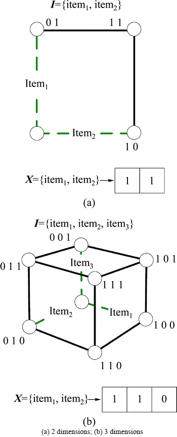
Fig. 2 Representing of search space, item sets and particles:

3.2 Initial particles and its dimensionality reduction

The quality of initial population has a big effect on frequent item sets mining from high-dimensional dataset. In BPSO-HD, the initial particles are firstly created randomly, and a part of them are modified by dimensionality reduction based on the following hypothesis.

Given an item set X, for IMG src="/web/fileinfo/upload/magazine/12542/311807/image018.jpg" onload="if(this.width>650){this.height=this.height*650/this.width;this.width=650;}">X_a, X_bX, the item sets X without X_a and X_b are respectively denoted by X–X_a and X–X_b. Based on Property 1, it is obviously that

from which, it can be deduced that

So, if Supp(X_a)≥Supp(X_b), Max Supp(X–X_b)≥ Max Supp(X–X_a).

Therefore, a hypothesis can be set that if Supp(X_a)≥ Supp(X_b), X–X_b has more probability to be a member of the top-k frequent item sets than X–X_a. Based on this hypothesis, if an initial particle X need to be modified, some dimensions of X whose supports are relatively lower than others will be removed. For example, given I={item₁, …, item₆} and X={item₁, …, item₃, item₅}, Fig. 3 shows the process of X’s dimensionality reduction.

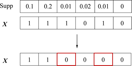
Fig. 3 Reduction of initial particle’s dimensionality

For an m dimensional dataset, the pseudo to generate initial population, Generate(m, n, pr), is shown as follows, where n is the size of population, X_i, P_i and v_i are respectively the i th particle, its local best solution and its velocity, pr is the proportion of initial particles to be modified and G_* is the global best solution.

Step 1: For i=1→n,

1) X_i←a random m dimensional binary vector.

2) While & Supp(X_i)==0 & |X_i|≥lmin, Xi←X_i–X′, where for item₁∈X′ and item₂∈X_i–X′, Supp(item₁)≤Supp(item₂).

3) P_i←X_i, v_i←0.

Step 2: G_*←0.

Step 3: Return X₁-X_n, P₁-P_n and v₁-v_n.

3.3 Updating positions of particles

The transfer function used for traditional BPSO is presented as Eq. (3), which is an S-shaped function, and the corresponding position updating equation is shown as Eq. (4). However, S-shaped transfer function has a drawback that particles are unchanged when their velocities increase [19]. Thus, BPSO-HD uses the V-shaped transfer function and its position updating rule [19-20].

The V-shaped transfer function and position updating rules are presented as Eqs. (5)-(6) and Fig. 4, where x_i^d(t) and v_i^d(t) indicate the position and velocity of the ith particle at iteration t in the dth dimension, (x_i^d(t))^-1 is the complement of x_i^d(t), and rand is a random values between 0 and 1.

                   (5)

           (6)

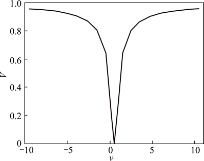
Fig. 4 V-shaped transfer function

For a dataset with m dimensions, the pseudo to update the positions of particles, UpdatePos(m, n, ω, c₁, c₂) is shown as follows, where w is the inertia weight, c₁ and c₂ are the acceleration coefficients, j₁ and j₂ are two random vectors, the values of which are between 0 and 1.

Step 1: For i=1→ n,

1) v_i←w·v_i+φ₁c₁×(P_i–X_i)+φ₂c₂×(G_*–X_i).

2) For d=1→m,

(1).

(2) If randi^d), x_i^d ←(x_i^d)^-1.

Step 2: Return X₁-X_n and v₁-v_n.

3.4 Fitness function and candidate results

Fitness function evaluates the qualities of particles. In BPSO-HD, the fitness of a particle is its support, namely,

Fitness(X)=Supp(X)                           (7)

However, to avoid two item sets in candidate results to be the same, and to ensure the length of results are more than a specified minimum length, the fitness function of a particle is modified into

       (8)

where l_min is the specified minimum length and R is the set of candidate results from previous mining. Every new G_* will be added into R.

Based on the fitness function, the pseudo to update local and global best solution, UpdateResult(n, l_min), is shown as follows.

Step 1: For i=1→n,

1) Fi←Fitness(X_i).

2) If Fi>Fitness(P_i), P_i ←X_i.

3) If Fi>Fitness(G_*),

(1) G_* ←X_i.

(2) R←R{G_*}.

Step 2: Return P₁-P_n and G_*

3.5 Dynamical dimensionality reduction of dataset

In frequent item sets mining, the high dimensionality always causes the large search space, which severely drags the performance of PSO-like methods. Thus, BPSO-HD designs a mechanism to reduce dimensionality dynamically.

Suppose that BPSO-HD is in one of the top-1 frequent set mining phases and G_* is the current best solution. From Property 1, given item′∈I and Supp(item′) < Supp(G_*), it can be known that for XI and item′∈X, Supp(X) is smaller than Supp(G_*). Thus, item′ is useless for this optimal search task and should be cut, and any particle will set item′ to 0, which is called dynamical dimensionality reduction of dataset.

Figure 5 shows an example of dynamical dimension reduction, where supports are beside vertices.

For a dataset with m dimensions, the pseudo to reduce dimensionality dynamically, Reduce(m, n), is shown as follows.

Step 1: For d=1→ m,

1) If Supp(item_d)*),

(1) For i=1→n, x_i^d← 0.

Step 2: Return X₁-X_n.

3.6 Whole pseudo of BPSO-HD

Based on the description above, for a dataset with m dimensions, the whole pseudo of BPSO-HD, BPSO-HD (k, N_i, m, n, pr, ω, c₁, c₂, l_min), is shown as follows, where N_i is the number of iteration of every top-1 frequent item set mining.

Step 1: For r=1→ k,

1) Generate(m, n, pr).

2) UpdateResult(n, l_min).

3) For i=1→N_i,

(1) UpdatePos(m, n, ω, c₁, c₂).

(2) Reduce(m, n).

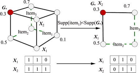
Fig. 5 Dynamically dimensionality reduction of dataset

(3) UpdateResult(n, l_min).

Step 2: Sort R by their fitness from high to low, and suppose the new sequence be R={R₁, R₂, …}.

Step 3: Return R₁-R_k.

4 Experiments and discussion

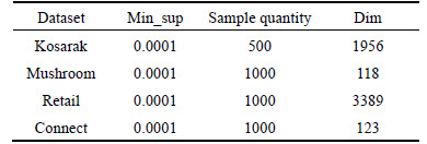
In this section, 4 sub-datasets sampled from datasets kosarak, mushroom, connect and retail are used to evaluate BPSO-HD, as shown in Table 1. The original datasets are downloaded from the website: http://fimi. ua.ac.be/data/. All experiments are conducted in Microsoft Windows XP using a compatible computer with an Inter i7 3.4 GHz CPU and a 3.49 GB RAM. Every algorithm is coded by Matlab and the m language.

Table 1 Sub-datasets used in experiments

4.1 Experiment 1

In experiment 1, BPSO-HD is compared with Apriori to test its reliability based on the 4 sub-datasets. For BPSO-HD, k=3, N_i=100, n=20, pr=0.3, w=0.5, c₁=c₂=1 and l_min=3. The min_sup of Apriori is set to 0.0001. For every dataset, both Apriori and BPSO-HD are run 100 times to mine the top-k frequent item sets.

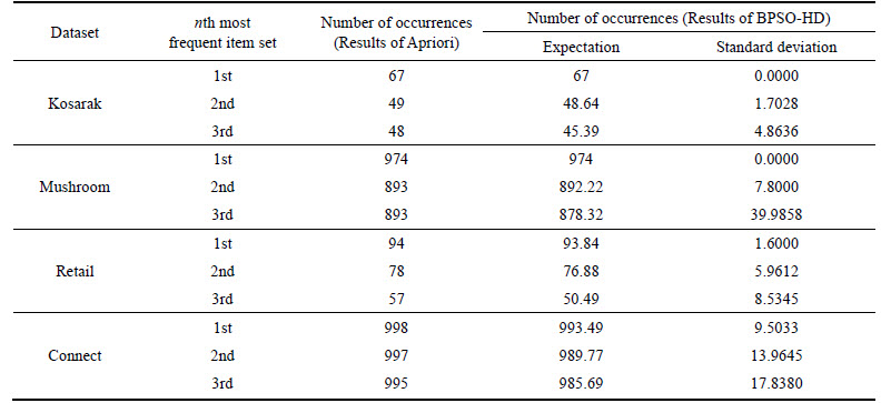
Figure 6 shows the occurrence times of the top-k frequent item sets generated by BPSO-HD and Apriori, where all the 1st, 2nd and 3rd most frequent item sets are sorted by their occurrence times from low to high. Table 2 shows the expectations and standard deviations of these results.

According to Fig. 6 and Table 2, it can be known that BPSO-HD can mine the exact top-k frequent item sets in most cases, the expectations of the results of BPSO-HD are close to the ones of Apriori and the standard deviations are low, which indicates that BPSO-HD has the high reliability.

However, whatever dataset based, the 1st most frequent item set generated by BPSO-HD is always the most precise, the 2nd most frequent item set is the 2nd most precise and the 3rd is the last one. The reason can be analyzed as follows.

Given a sequence {p₁, p₂, …, p_k} which represents the probabilities of the top-k frequent item sets to be mined out by BPSO, it can be assumed that p₁≥p₂…≥p_k. Meanwhile, suppose {p′₁, p′₂, …, p′_k} are the probabilities of the top-k frequent item sets which can not be mined out by k times of BPSO, it can be known that

p′₁=(1– p₁)^k,

p′₂=(1–p₂)^k,

p′₃=(1–p₃)^k,

and it is also obviously that p′₁≤p′₂, …, ≤p′_k, which means that based on BPSO, the higher fitness results in the higher probability to be mined out. Because BPSO-HD is modified from BPSO, it also inherits this characteristic.

4.2 Experiment 2

In experiment 2, BPSO-HD is compared with BPSO and BPSO with Generate(m, n, pr) called BPSO with reasonable initial population (BPSO-RI) to prove that the improvements in BPSO-HD are meaningful. For BPSO-HD, BPSO and BPSO-RI, N_i=100, n=20, w=0.5, c₁=c₂=1 and l_min=3. The pr of BPSO-HD and BPSO-RI are both 0.3, and the k of BPSO-HD is 1. To be fair, every algorithm uses the V-shaped transfer function and Eq. (8) to be the fitness function. All algorithms are run 100 times to mine the most frequent item sets based on every dataset.

Figure 7 shows the occurrence times of the top-1 frequent item sets generated by BPSO-HD, BPSO and BPSO-RI, where the results are sorted through their occurrence times from low to high.

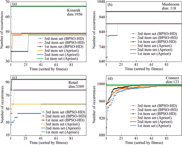
Fig. 6 Results of BPSO-HD compared with results of Apriori based on kosarak (a), mushroom (b), retail (c) and connect (d)

Table 2 Expectations and standard deviations of occurrence times of results generated by BPSO-HD

According to Fig. 7, it can be known that when facing some high dimensional datasets, the ordinary BPSO almost totally loses its power, and when Generate(m, n, pr) is applied, the performance of BPSO has some progress but also drags behind BPSO-HD. The reasons are analyzed by follows.

1) The high dimension results in the large search space, which extremely reduces the search efficiency of ordinary BPSO and makes it almost lose power.

2) Generate(m, n, pr) enhances the qualities of the initial population, which is very helpful to improve search performance, but with a large search space generated by high dimension, particles also have high probabilities to go some useless area by random flying.

Therefore, just only the good initial population is not enough to make search efficiency satisfactory.

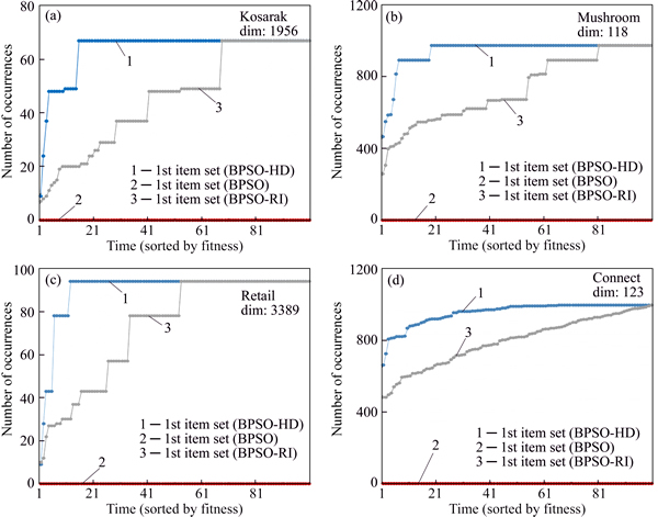
Fig. 7 Results of BPSO-HD compared with results of BPSO and BPSO-RI based on kosarak (a), mushroom (b), retail (c) and connect (d)

3) The Generate(m, n, pr) and Reduce(m, n) of BPSO-HD not only give a reasonable initial population, but also reduce the probabilities of particles to go useless areas, both of them enhance the performance remarkably, so the performance of BPSO-HD is better than the performances of BPSO and BPSO-RI.

4.3 Experiment 3

In experiment 3, BPSO-HD is compared with quantum swarm evolutionary (QSE), QSE with Generate(m, n, pr) called QSE with reasonable initial population (QSE-RI) and BPSO-RI to prove that the BPSO-HD is better, and the traditional way to modify PSO algorithm, which enhances the randomness of particles, is not suitable for the high-dimensional datasets. For BPSO-HD, k=1, pr=0.3, N_i=100, n=20, w=0.5, c₁=c₂=1 and l_min=3. The parameters of QSE are the same as what are set in MOURAD’s thesis [4], and pr of QSE-RI is 0.3. The parameters of BPSO-RI are the same as experiment 2. To be fair, all the algorithms use Eq. (8) to be the fitness function, and all of them are run 100 times to mine the most frequent item sets based on every dataset.

Figure 8 shows the occurrence times of the top-1 frequent item sets generated by BPSO-HD, QSE, QSE-RI and BPSO-RI, where all the results are sorted by their occurrence times from low to high.

According to Fig. 8, it can be known that like BPSO, when facing some high dimensional datasets, QSE also almost loses its power, and when Generate(m, n, pr) is used, its performance has some progress but also drags behind BPSO-HD. In the other hand, except the dataset retail, QSE-RI has not presented any advantage when compared with BPSO-RI. The reasons are analyzed as follows.

1) As analyzed in Experiment 2, the high dimensionality extremely reduces the efficiency of QSE, and even a good initial population is not enough to make the results of QSE-RI satisfactory. However, through Generate(m, n, pr) and Reduce(m, n), BPSO-HD has both reasonable initial population and the dynamically reducing search space, which ensures its high performance and makes it better than QSE and QSE-RI.

2) The strengthened randomness of particle in QSE is not only trivial when facing the huge search space generated by high dimensionality, but also reduces the convergence of algorithm. Thus, except a tiny advantage on retail, QSE-RI not only has shown any advantage to BPSO-RI, but also performs worse than BPSO-RI on connect.

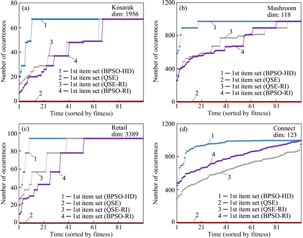
Fig. 8 Results of BPSO-HD compared with results of QSE, QSE-RI and BPSO-RI based on kosarak (a), mushroom (b), retail (c) and connect (d)

5 Conclusions

1) The traditional improvement method by enhancing randomness of particles in some PSO-like algorithms such as QSE is not suitable to mine the frequent item sets from high-dimensional datasets.

2) The dimensionality reduction of initial particles and dynamical dimensionality reduction of datasets are helpful for PSO-like algorithms to mine the frequent item sets from high-dimensional datasets, both of which have broad and great research prospects.

3) BPSO-HD, based on dimensionality reduction of initial particles and dynamical dimensionality reduction of datasets, is reliable and generates results more precise than other PSO-like algorithms such as BPSO and QSE to mine the frequent item sets from high-dimensional datasets.

References

[1] HAN Jia-wei, PEI Jian, KAMBER M. Data mining: Concepts and techniques [M]. Third Edition. Elsevier, 2011: 243-262.

[2] LUO Ke, WANG Li-li, TONG Xiao-jiao. Mining association rules in incomplete information systems [J]. Journal of Central South University, 2008, 15: 733-737.

[3] ALATAS B, AKIN E. Rough particle swarm optimization and its applications in data mining [J]. Soft Computation, 2008, 12: 1205-1218.

[4] YKHLEF M. A quantum swarm evolutionary algorithm for mining association rules in large databases [J]. Journal of King Saud University-Computer and Information Sciences, 2011, 23: 1-6.

[5] ANKITA S, SHIKHA A, JITENDRA A, SANJEEV S. A review on application of particle swarm optimization in association rule mining [J]. Advances in Intelligent Systems and Computing, 2013, 199: 405-414.

[6] XU Yang, ZENG Ming-ming, LIU Quan-hui, WANG Xiao-feng. A genetic algorithm based multilevel association rules mining for big datasets [J]. Mathematical Problems in Engineering, 2014: 867149.

[7] BILAL A, ERHAN A. An efficient genetic algorithm for automated mining of both positive and negative quantitative association rules [J]. Soft Computation, 2006, 10: 230-237.

[8] KUO R J, SHIH C W. Association rule mining through the ant colony system for national health insurance research database in Taiwan [J]. Computers and Mathematics with Applications, 2007, 54: 1303-1308.

[9] KENNEDY J, EBERHART R C. Particle swarm optimization [C]// LOZOWSKI A, CHOLEWO T J, ZURADA J M. Proceedings of the IEEE International Conference on Neural Networks. Perth, Australia: IEEE press, 1995: 2147-2156.

[10] KUO R J, CHAO C M, CHIU Y T. Application of particle swarm optimization to association rule mining [J]. Applied Soft Computing, 2011, 11: 326-336.

[11] BOHANEC M, RAJKOVIC V. DEX: An expert system shell for decision support [J]. Sistemica, 1990, 1(1): 145-157.

[12] BADAWY O M, SALLAM A A, HABIB M I. Quantitative association rule mining using a hybrid PSO/ACO algorithm (PSO/ACO-AR) [C]// JAMEL F. Proceedings of Arab Conference on Information Technology. Hammamet, Tunisia: CCIS Press, 2008: 1-9.

[13] KABIR M M J, XU S X, KANG B H, ZHAO Z Y. Association rule mining for both frequent and infrequent items using particle swarm optimization algorithm [J]. International Journal on Computer Science and Engineering, 2014, 6(7): 221-231.

[14] SALAM A, KHAYAL M S H. Mining top-k frequent patterns without minimum support threshold [J]. Knowledge Information System, 2012, 30: 57-86.

[15] BANKS A, VINCENT J, ANYAKOHA C. A review of particle swarm optimization [J]. Nat Computation, 2007, 6: 467-484.

[16] POLI R, KENNEDY J, BLACKWELL T. Particle swarm optimization an overview [J]. Swarm Intelligent, 2007, 1: 33-57.

[17] KENNEDY J, EBERHART R C. A discrete binary version of the particle swarm algorithm [C]// JAMES M T. Proceedings of the Conference on Systems, Man, and Cybernetics. Florida, USA: IEEE Press, 1997: 4104-4108.

[18] CLERC M. Discrete particle swarm optimization, illustrated by the traveling salesman problem [J]. Studies in Fuzziness & Soft Computing, 2004, 47(1): 219-239.

[19] MIRJALILI S, LEWIS A. S-shaped versus V-shaped transfer functions for binary particle swarm optimization [J]. Swarm and Evolutionary Computation, 2013, 9: 1-14.

[20] MIRJALILI S, MIRJALILI S M, YANG X S. Binary bat algorithm [J]. Neural Computation and Application, 2014, 25(3): 663-681.

(Edited by FANG Jing-hua)

Received date: 2015-04-20; Accepted date: 2015-09-17

Corresponding author: HUANG Jian, Professor, PhD; Tel: +86-13973166586; E-mail: huang_jian@139.com