Trans. Nonferrous Met. Soc. China 28(2018) 2607-2618

Volatility-volume relationship of Chinese copper and aluminum futures market

Bai-sheng SHI¹, Xue-hong ZHU^1,2, Hong-wei ZHANG¹, Yi ZENG¹

1. School of Business, Central South University, Changsha 410083, China;

2. Institute of Metal Resources Strategy, Central South University, Changsha 410083, China

Received 22 March 2018; accepted 6 July 2018

Abstract: Following Bessembinder and Seguins, trading volume is separated into expected and unexpected components. Meanwhile, realized volatility is divided into continuous and discontinuous jump components. We make the empirical research to investigate the relationship between trading volume components and various realized volatility using 1 min high frequency data of Shanghai copper and aluminum futures. Moreover, the asymmetry of volatility-volume relationship is investigated. The results show that there is strong positive correlation between volatility and trading volume when realized volatility and its continuous component are considered. The relationship between trading volume and discontinuous jump component is ambiguous. The expected and unexpected trading volumes have positive influence on volatility. Furthermore, the unexpected trading volume, which is caused by arrival of new information, has a larger influence on price volatility. The findings also show that an asymmetric volatility-volume relationship indeed exists, which can be interpreted by the fact that trading volume has more explanatory power in positive realized semi-variance than negative realized semi-variance. The influence of positive trading volume shock on volatility is larger than that of negative trading volume shock, which reflects strong arbitrage in Chinese copper and aluminum futures markets.

Key words: nonferrous metals futures; volatility-volume relationship; high frequency data; trading volume; asymmetry

1 Introduction

After nearly 20 years of development, Chinese nonferrous metal futures market has become an important metal futures trading place, whose trading volume is second only to the London Metal Exchange (LME). Nonferrous metals also occupy an important strategic position in China’s national economy. Among them, copper and aluminum are called “industrial food” and are widely used in various fields of the national economy. Under the background of financialization, the unpredictable price of nonferrous metals has brought difficulties to the daily observation and policy formulation to government regulatory authorities, while the trading volume is easy to observe and can be used as a proxy variable for market information flow. Therefore, by observing the change in the volume of this dominant indicator, we can predict the trend of market price changing and avoid risks effectively. Hence, research on volatility-volume relationship of nonferrous metals futures market has become an important topic.

Due to the noise in the market, many practical problems cannot be explained by traditional financial theory. The research on volatility-volume relationship provided new ideas for scholars’ research. CROUCH and ROBERT [1] found a positive correlation between trading volume and absolute return in the stock market. By establishing the model, CLARK [2] proved the positive correlation between price volatility and volume in financial markets, and proposed a famous theory: Mixture Distribution Hypothesis (MDH). COPELANG and ANALYSIS [3] built the continuous information arrival model and found that the information will gradually disperse after it reaches the market, causing changes in market prices and volume. KARPOFF and ANALYSIS [4] proposed that the relationship between volume and price involves the reaching rate, reaching path and the degree of communication.

In order to find out the main driving factors behind the relationship between volatility and volume, scholars began to analyze the quantitative relationship of volatility-volume from a more micro perspective.  KYLE [5] assumed that there are three types of traders on the market: informed traders, market makers, and random flow traders. ADMATI and PFLEIDERER [6] proposed that there is still a fourth trader in the market who has certain judgment on market timing, namely free-flow trader. HE et al [7] investigated the effect of investor risk compensation (IRC) on stock market  returns, and the results show that current IRC has a significant and positive effect on stock returns. BESSEMBINDER et al [8] decomposed volume into expected volume and unanticipated trading volume, and found that unexpected volume is the main factor leading to stock price fluctuations. WEN et al [9,10] found that investors’ risk preference characteristics play a significant role in stock market prices. CHENG et al [11] showed that long memory feature with a certain period exists in volatility-volume correlation. KARAA et al [12] investigated the impact of trading intensity and trading volume on return volatility by using transaction data from the Tunis Stock Exchange. MAGKONIS and TSOUKNIDIS [13] examined the existence of dynamic spillover effects across petroleum spot and futures volatilities, trading volume and open interest. With the development of computer technology and the degree of informatization, the realized volatility based on high frequency data is applied to the empirical study of volatility-volume relationship. CHAN and FONG [14] used realized volatility obtained by summing up intraday squared returns to confirm that number of trades is the dominant factor behind the volatility-volume relation. Besides, using high-frequency data, WEN et al [15] and GONG et al [16] applied the realized volatility to forecast the volatility and investigate the risk-return trade-off for crude oil futures. In view of the nonferrous metal futures market, some scholars have adopted different methods to study the volatility prediction and leverage effects of the nonferrous metal futures market based on high-frequency data [17-19]. However, they didn’t do further exploring on the relationship between the decomposition of realized volatility and volume from a more microscopic perspective. ANDERSEN et al [20] separated the continuous sample path variance and the jump variance of the realized volatility based on the quadratic variation theory. Based on this research, some scholars conducted empirical studies on the correlation among continuous fluctuation components, jump components and volume [21]. Followed by the research foundation of GIOT et al [22], CHEVALLIER and  Sévi [23] explored the asymmetry of the relationship between volume and price in the energy futures market. SLIM and DAHMENE [24] decomposed the transaction volume into informed trading volume and liquidity trading volume, and further explored the correlation between the decomposition of the CAC40 stock volume and the decomposition of the volatility of Paris Stock Exchange, but did not continue to explore whether there is asymmetry in the volatility-volume relationship of financial market. XIAO et al [25] used the positive and negative changes of the crude oil volatility index (OVX) and examined the asymmetric effects of uncertainty shocks. Todorova and CLEMENTS [26] found that both trading volume and trading frequency are highly relevant. However, they did not further study the asymmetry of volatility-volume relationship based on the trading volume.

In view of the contributions and shortcomings of the above literature research, this work decomposes the trading volume into the predictable and unpredictable parts, and decomposes the high-frequency realized volatility into continuous volatility and jumps. Further, the relationship between the decompositions of volume of Chinese copper and aluminum futures market and the decompositions of realized volatility is studied. Moreover, the asymmetry of volatility-volume relationship in Chinese copper and aluminum futures market was explored.

The main innovations of this work are as follows: firstly, the research on commodity futures, especially the nonferrous metal futures market, is very rare in the existing research, while nonferrous metals like copper and aluminum have a vital position in China’s industrial structure and national economy. Secondly, most of the research on volatility-volume relationship was focused on correlation test and causal analysis, but this work further decomposes the trading volume into the expected volume and the unexpected volume, and discusses the relationship between price volatility and volume from the market microstructure. Thirdly, existing literature is mostly based on daily data instead of high frequency  data, while Avramov et al [27] found that the research based on high frequency data can significantly improve the explanatory ability of the model. Finally, this work further explores the asymmetry of the volatility-volume relationship in Chinese copper and aluminum futures market.

2 Methodology

2.1 Volatility estimation

2.1.1 Realized volatility

Andersen and Bollerslev [28] proposed the realized volatility for measuring the return volatility in the financial market. For a given day t, the daily realized volatility can be computed as

                                   (1)

where r_t,i is the ith return (i=1, …, M) at the given day t, i.e., r_t,i=100(lg P_t,i-lg P_t,i-1), and P_t,i is the ith closing price at the given day t.

2.1.2 Jump and continuous variations

We assume that the logarithmic price of copper and aluminum futures (p_t=lg P_t) within the trading day follows a general stochastic volatility jump diffusion model:

               (2)

where μ_t is the drift term with a continuous variation sample path; σ_t denotes a strictly positive stochastic volatility process; W_t is the driving standard Brownian motion; κ_tdq_t denotes the random jump size.

For discrete prices process, the return volatility at the given day t includes jump variation, so it is not an unbiased estimator of integrated volatility. The return volatility at the given day t is measured by the quadratic variation:

                        (3)

where  is the continuous sample path variation. denotes the discontinuous jump variation in [t-1, t].

When M→∞, the daily realized volatility can be used as a consistent estimator of quadratic variation τ_t:

              (4)

Following Barndorff et al [29,30], the continuous sample path variation  can be estimated by the realized bipower variation :

                   (5)

where, and Z_t is a random variable which drives a standard normal distribution. Following Barndorff et al [29,30] and HUANG and TAUCHEN [31], Z-statistics is used to identify the discontinuous jump variation:

  (6)

where , and ω_t denotes the realized tri-power quarticity,

Based on the above jump detection test statistic, we obtain the daily discontinuous jump variation J_t:

                       (7)

and the daily continuous sample path variation C_t:

              (8)

where I is the indicator function and Φ_α refers to the critical value from the standardized normal distribution. Following GONG et al [16] and ANDERSEN et al [32], we use a critical value of α=0.99.

2.1.3 Realized semi-variances

Barndorff et al [33] developed the daily realized semi-variances which can capture the variation only according to negative or positive return in intraday trading. The daily positive realized semi-variance estimator is defined as

                        (9)

And the daily negative realized semi-variance estimator is written as

                        (10)

2.2 Analysis of volatility-volume relationship

Considering the complexity of price volatility in the futures market, regression models are established from three different aspects: the basic volatility-volume relationship, the volatility-volume relationship with volume decomposition, and the asymmetric volatility- volume relationship. Further, comprehensive survey of price volatility in Chinese copper and aluminum futures market is conducted.

2.2.1 Basic volatility-volume relationship model

The basic volatility-volume relationship model mainly discusses the relationship of volatility and its decomposition part with trading volume. First, referring to the Realized Bipower Variation proposed by Barndorff and Shephard [29], the realized volatility is decomposed into the continuous part and the jumping part, and further the week dummy variable is introduced to discuss the “week effect” of new information release on the price volatility of nonferrous metal futures. At the same time, emulating the modeling methods of GIOT et al [22], Chevallier and    Sévi [23] and SLIM and Dahmene [24], we select the continuous lag of 12 orders to eliminate the autocorrelation of realized volatility and the continuous part. The basic volatility-volume relationship model is as follows:

  (11)

 (12)

             (13)

where C_i,t is the realized volatility of futures i on day t, and the realized volatility is defined as the sum of the squares of intraday high-frequency gains. C_i,t and J_i,t  are the continuous variation and jump variation based on the realized double power variation (RBV) decomposition, respectively. V_i,t is the trading volume; DUMMY_i,t is the intra-week dummy variable that takes into account the impact of new information released in the copper and aluminum futures market. In this work, the dummy variable of Wednesday is used, and ε_i,t represents the random error term.

2.2.2 Volatility-volume relationship model with volume decomposition

In this section, we mainly discuss the impact of expected trading volume (non-information volume) and unexpected trading volume due to arrival of new information on price volatility. It is known from existing research that foreign information can cause financial asset price volatility, which is based on certain assumptions: investors cannot predict future information. It can be seen that the expected trading volume and the unexpected trading volume have different effects on price volatility. Therefore, it is necessary to decompose the volume and explore the relationship between the trading volume decompositions and price volatility from a more microscopic perspective.

After the logarithm of the trading volume data of copper and aluminum futures, the autocorrelation test is carried out. It can be found that there is a high autocorrelation between the trading volume sequences of the two metal futures. In order to eliminate the autocorrelation of sequences, the regression of trading volume sequences is conducted by using the autoregressive moving average model ARMA(p,q):

                 (14)

The expected trading volume is the fitting value calculated by model ARMA(p,q), denoted as . The unexpected trading volume is the value of the volume after eliminating the sequence correlation, that is, the estimated value of the regression residual. It is also the difference between the actual value and the fitting value, denoted as . Selection of lag order in model ARMA(p,q) is based on AIC criterion and SC criterion. The expected and unexpected trading volumes were introduced into the basic model as explanatory variables, and the following formula can be obtained:

                      (15)

                      (16)

      (17)

where  and  respectively represent the expected trading volume and unexpected trading volume for future i in the day t.

2.3 Asymmetric volatility-volume relationship model

The asymmetric relationship between trading volume and price volatility in Chinese copper and aluminum futures market is further discussed. The effects of trading volume on positive and negative realized semi-variances, and the different impact of positive and negative trading volume on price volatility are discussed.

From the perspective of realized volatility, the impact of upside (positive) and downside (negative) risks of prices on investors’ trading strategies was studied. Barndorff et al [30] proposed the concepts of daily positive realized semi-variance and daily negative realized semi-variance  for realized volatility. CHEVALLIER and Sévi [23] applied the daily positive and negative realized semi-variances to the asymmetric study of the relationship between price volatility and volume. With reference to their research results, the following model is constructed in this work:

                       (18)

where;  and  indicate the daily positive and negative realized semi-variances, respectively.

From the perspective of trading volume, the different impact of positive and negative unexpected trading volume on the price volatility of futures market is studied. Based on the volume decompositions, a positive unexpected trading volume is introduced, and the following model is constructed:

                     (19)

where the unexpected trading volume >0, β_2i=1; or β_2i=0.

In order to eliminate the possible autocorrelation or heteroscedasticity of the model estimation results, OLS with Newey West estimation method is used to estimate the parameters in all the empirical models except the jump volatility, and TOBIT regression is adopted to estimate the jump volatility with reference to GIOT et al [22].

3 Empirical analysis

Two most typical nonferrous metal futures in China are taken as study objects: copper futures and aluminum

futures, and the 1 min closing prices of copper and aluminum futures due in three months in Shanghai futures exchange are selected, whose trading volume of copper and aluminum futures is the largest in China. The sample interval is selected from July 1, 2010 to July 1, 2015 (excluding holidays, a total of 1214 trading days). The trading hours are 8:59 to 11:29 a.m. and 13:30 to 15:00 p.m., a total of 227 intervals per day, namely M=227. The selected sample indexes are trading time, closing price, opening price and trading volume, all of which are from CSMAR database (http://www.gtarsc. com/) [34]. The data processing software is MATLAB2017a and STATA14.0. Sample data selection, descriptive statistics and empirical results are then analyzed.

Fig. 1 Realized volatility (a), trading volume (b), continuous (c) and discontinuous jump (d) components of copper futures from July 1, 2010 to July 1, 2015

Fig. 2 Realized volatility (a), trading volume (b), continuous (c) and discontinuous jump (d) components of aluminum futures from July 1, 2010 to July 1, 2015

Based on Section 2, the daily return r_t, realized volatility RV_t and its continuous variation C_t and jump variation J_t are calculated. In order to better analyze the characteristics of different components that make up the total daily return variation for copper and aluminum futures markets, Figs. 1 and 2 are plotted. The figures clearly illustrate that for copper or aluminum futures, each component exhibits volatility clustering, which indicates rather distinct dynamic dependence in each of the different components.

3.1 Descriptive statistics of sample data

Descriptive statistics of various indicators for copper and aluminum futures are recorded in Table 1 and Table 2. The skewness and kurtosis of the volatility and decomposition sequence of copper and aluminum futures show that the price volatility has a significant peak and tail. Except the jump part and the unexpected volume of aluminum futures, each statistic has a high degree of autocorrelation with a lag of 12 orders. Besides, the results of ADF unit root test prove that all indicators are stationary. Specifically, the proportion of continuous component of realized volatility in copper and aluminum futures is larger than that of the jump component (continuous components account for 88.5% and 70.6% for copper and aluminum futures, respectively), indicating that the continuous component in the realized volatility occupies the dominant position, while the effect of the jump component is relatively small. In addition, the mean of the daily positive and negative realized semi-variances (and ) is nearly the half of the realized volatility, and the mean of negative realized semi-variance is greater than the mean of positive realized semi-variance. This indicates that the risk of price decline in the copper and aluminum futures market is higher than the risk of price rise. It is also indirectly reflected that the trading strategies of investors in the two markets tend to short-selling, and they are relatively cautious about the long market.

3.2 Empirical results and analysis

Based on the descriptive and correlation analysis of various indicators, the relevant data of the copper and aluminum futures market are used to demonstrate the model. Only the parameter estimation results of main variables are listed here, and the analysis is carried out based on the reality of the nonferrous metal futures market.

Table 1 Descriptive statistical analysis of various indicators for copper futures in China

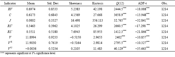
Table 2 Descriptive statistical analysis of various indicators for aluminum futures in China

3.2.1 Basic volatility-volume relationship model

Tables 3 and 4 show the estimation results for the basic volatility-volume relationship model of copper and aluminum futures.

Considering that the volatility-volume relationship model of jump variation uses the TOBIT regression method, the value of its goodness of fit is meaningless, so it is represented by NA. The results of Table 3 show that the trading volume of copper futures market has a positive impact on the realized volatility and the continuous volatility, and the impact is significant at the significance level of 1%. Similar results exist in the aluminum futures market (see Table 4). This indicates that the price volatility of copper and aluminum futures increase with the increase of trading volume, and slow down with the decrease of trading volume. This means that both the “volatility and volume rise together” and “volatility and volume fall together” exist in the two futures markets of copper and aluminum. The dummy variable of Wednesday, which represents the new information released during the week, has significant influence on the realized volatility and continuous volatility of copper and aluminum futures markets, and all coefficients are negative (the RV and C coefficients for copper futures are -0.105 and -0.0528, respectively, and for the aluminum futures coefficients are -0.0554 and -0.0385, respectively). It is shown that realized volatility and its continuous component in the copper and aluminum futures are obviously negatively affected by the week effect. That is to say, the week effect has a certain “absorption” effect on the price volatility and its continuous component of the copper and aluminum futures markets. At the same time, the corresponding parameters of the dummy variables on the jump volatility are not significant, indicating that the week effect has no significant effect on the jumps. The performances of the impact on trading volume for the jump variations are different between the copper and aluminum futures market. In the copper futures market, the trading volume has no significant impact on the jump variation, but has a significant impact on the aluminum futures market. In Table 3 and Table 4, the adjusted R² of the continuous variation is higher than that of the realized volatility, indicating that after removing the jump variation, the adjustment and goodness of the basic volatility-volume relationship model are significantly improved, which reflects the volatility-volume relationship in copper and aluminum futures is affected by the noise caused by the jump component of volatility.

3.2.2 Volatility-volume relationship model with volume decomposition

Table 5 and Table 6 show the estimation results of the volatility-volume relationship model with volume decomposition. It can be seen from Table 5 that the unexpected trading volume has a significant positive influence (at the 1% significance level) on realized volatility and its continuous part, while the coefficient corresponding to the expected volume is not significant. In the aluminum futures market, both the expected and unexpected volume have a significant positive impact on the realized volatility and its continuous and jump decompositions (at the 1% significance level). In addition, the coefficient of unexpected volume is greater than that of expected volume (0.326>0.190 for realized volatility, 0.262>0.141 for continuous volatility, and 0.052>0.023 for jump volatility). It can be concluded that the impact of unexpected trading volume on volatility in the copper and aluminum metal futures market is greater than that of expected trading volume on volatility. The unexpected trading volume represents the information volume caused by the newly arrived market information, while the expected trading volume represents the non-information volume caused by the market development, investor position adjustment or liquidity demand. This indicates that non-information trading volume has less driving force for price volatility in copper and aluminum futures market, and investors will refer to the information of new arrival in the market when making investment strategies more, which is consistent with the conclusion of Bessembinder et al [8]. The parameters of dummy variables representing the week effect for the realized volatility, and its continuous component are significant and negative for copper and aluminum futures market. This suggests that the copper and aluminum futures markets are negatively affected by the week effect. In addition, from the perspective of adjusted R², after removing the jump volatility, the adjusted goodness of fit of volatility-volume relationship model based on the volume decomposition is also significantly improved.

3.2.3 Asymmetric volatility-volume relationship model

The asymmetric volatility-volume relationship model is mainly manifested in the asymmetry of the realized volatility and the asymmetry of trading volume. The estimated results are given in Table 7 and Table 8.

Table 3 Estimation results of basic volatility-volume relationship model for Chinese copper futures

Table 4 Estimation results of basic volatility-volume relationship model for Chinese aluminum futures

Table 5 Estimation results of volatility-volume relationship model with volume decomposition for copper futures

Table 6 Estimation results of volatility-volume relationship model with volume decomposition for aluminum futures

Table 7 Estimation results for asymmetric volatility-volume relationship model of aluminum futures in China

Table 8 Estimation results for asymmetric volatility-volume relationship model of copper futures in China

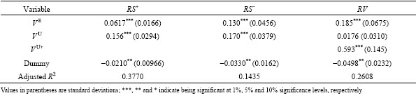
First, the asymmetry of realized volatility is considered. As shown in Table 7, the expected trading volume of copper futures market has no significant impact on the positive realized semi-variances, and has a significant positive impact on the negative realized semi-variances (at the 10% significance level). The unexpected trading volume has a significant positive effect on the positive and negative realized semi-variances (under the significance level of 1%), but the corresponding coefficient of the negative realized semi-variance (0.119) is larger than that of the positive realized semi-variance (0.112). In the aluminum futures market, both the expected and unexpected trading volumes have significant positive effects on the positive and negative realized semi-variances (at the significance level of 1%), and the corresponding coefficients of the negative realized semi-variances are greater than those of the positive realized semi-variances (expected volume: 0.130>0.0617; unexpected volume: 0.170>0.156). It can be concluded that in the copper and aluminum futures markets in China, the impact of volume decomposition on the negative realized semi-variance is greater than that of the positive realized semi-variance. This indicates that when the price volatility in the market is negative, the price volatility caused by the trading volume change is larger. However, looking at the adjusted R² corresponding to Table 7 and Table 8, the adjusted R² of positive realized semi-variances for the volatility- volume relationship model are significantly greater than that of negative realized semi-variances for the volatility-volume relationship model (0.4868>0.3533 for copper futures and 0.3370>0.1435 for aluminum futures). It is indicated that the volume decomposition has stronger interpretation ability for the positive realized semi-variance, and it is also indirectly indicated that the positive realized semi-variance contains more volatility-volume relationship information than the negative realized semi-variance. This is contrary to the research conclusions of POTTON and SHEPPARD [35].

Secondly, the asymmetry of trading volume is considered. Since the above-mentioned unexpected volume has a greater impact on the price volatility of the futures market, the unexpected trading volume is selected to perform the positive and negative impact test, and the dummy variable β_2i is introduced into the parameter estimation. When the unexpected trading volume is positive, β_2i=1, otherwise β_2i=0. It can be seen from Table 7 that the dummy variable coefficient corresponding to the positive unexpected trading volume is significantly positive (at the significance level of 10%) in the copper futures market, and is greater than the corresponding coefficient of the unexpected trading volume and the expected trading volume (0.203> 0.124>0.0419). In the aluminum futures market, the dummy variable coefficient corresponding to the positive unexpected trading volume is significantly positive (at the significance level of 1%), and is much larger than the corresponding coefficient of the expected trading volume (0.593>0.185) (see Table 8). It can be inferred that in Chinese copper and aluminum metal futures market, the impact of positive trading volume shock on price volatility is greater than that of negative trading volume shock on price volatility, and the impact of positive trading volume shock on price volatility is greater than that of negative trading volume shocks on price volatility. This shows that when the futures investors in China make trading decisions, the information of the increasing volume is more affected than the information of the shrinking volume, that is, investors are more sensitive to the “good” news than the “bad” news. This reflects from the side that copper and aluminum metal futures investors are speculative in trading.

4 Robustness test

We use other methods to verify the robustness of the above-mentioned volatility-volume relationship, for example, using different jump test thresholds (such as at 5% and 0.1% significance levels), using a more robust jump test estimator MedRV to replace RBV(υ_t), denoted as γ, or adopting different jump check thresholds for MedRV. In this work, the estimation results of using the more robust jump test estimator MedRV are given only.

When the sampling frequency does not tend to be infinite (as is often the case in empirical tests), price volatility tends to be positive-biased, because volatility has the characteristics of volatility aggregation, and a large volatility is usually not followed by a small one. In order to reduce the conditional heteroscedasticity that may occur in the above empirical results, in this work, with reference to the research ideas of ANDERSEN et al [36], a new estimator MedRV is used as an indicator to measure the robust estimate of jump volatility to replace RV(C), and the estimation is re-evaluated. Among them,

             (20)

Accordingly, ω_i,t in the Z_t statistic will also be replaced by MedRTO_i,t, denoted as δ_i,t:

             (21)

When δ_i,t statistic is significant, jump volatility can be expressed by

              (22)

With jump volatility, the continuous volatility part is easily expressed by the difference between the realized volatility and jump part. Based on the re-estimation, new estimation results are given in Table 9 and Table 10. From the estimation results, although there are some differences from the perspective of quantitative analysis, the qualitative result analysis is consistent with the result analysis obtained by using the realized bipower  variation, so the robustness of the volatility-volume relationship is verified.

Table 9 Estimated results of Chinese copper futures robustness test (MedRV)

Table 10 Estimated results of Chinese aluminum futures robustness test (MedRV)

5 Conclusions

1) There is a clear positive correlation between the price volatility and the trading volume in Chinese copper and aluminum futures markets. Affected by the macroeconomic situation and the demand of market, the price volatility of Chinese copper and aluminum futures market is quite frequent, but it maintains a certain degree of correlation with the trading volume. Investors can judge the possible risks in the market by observing the changes in trading volume and its decomposition indicators.

2) The influence degree of trading volume on different volatility component of copper and aluminum futures is different. Compared with the jump component, the continuous component of nonferrous metal futures contains more information. The correlation between trading volume and continuous component is closer; therefore, it is more accurate to predict the market volatility by using the continuous volatility information.

3) The trading volume can be used as a substitute for market information, but the impacts of different volume indicators on market price volatility are different. The expected trading volume has a limited ability to interpret price volatility. However, the unexpected trading volume has a stronger driving effect, and can explain market price volatility more strongly.

4) The impact of trading volume on price volatility in copper and aluminum futures markets are asymmetric. The positive volume shock is more influential than the negative volume shock, indicating that the investors are more sensitive to “good” news than “bad” news.

5) The management should strengthen the supervision on the market, and pay more attention to the changes in trading volume. On one hand, regulators should timely predict the price volatility that may be caused by the trading volume changing, and on the other hand, investors should also be alert to the changes of trading volume in the nonferrous metal futures. Furthermore, relevant departments should strengthen the risk aversion mechanism to prevent the financial crisis and prevent systemic risks.

References

[1] CROUCH, ROBERT L. The volume of transactions and price changes on the New York Stock Exchange [J]. Financial Analysis Journal, 1970, 26(4): 104-109.

[2] CLARK P. A subordinated stochastic process model with finite variance for security prices [J]. Econometrica: Journal of the Econometric Society,1973, 41(1): 157-159.

[3] COPELAND T, ANALYSIS Q. A probability model of asset trading [J]. Journal of Financial and Quantitative Analysis, 1977, 12(4): 563-578.

[4] KARPOFF J, ANALYSIS Q. The relation between price changes and trading volume: A survey [J]. Journal of Financial and Quantitative Analysis, 1987, 22(1): 109-126.

[5] KYLE A S. Continuous auctions and insider trading [J]. Econometrica: Journal of the Econometric Society, 1985, 53(6): 1315-1335.

[6] ADMATI A R, PFLEIDERER P. A theory of intraday patterns: Volume and price variability [J]. The Review of Financial Studies, 1988, 1(1): 3-40.

[7] HE Zhi-fang, HE Lin-jie, WEN Feng-hua. Risk compensation and market returns: The role of investor sentiment in the stock market [J]. Emerging Markets Finance and Trade, 2019, 55(3): 704-718. DOI:10.1080/1540496X.2018.1460724.

[8] BESSEMBINDER H, SEGUIN P, ANALYSIS Q. Price volatility, trading volume, and market depth: Evidence from futures markets [J]. Journal of Financial and Quantitative Analysis, 1993, 28(1): 21-29.

[9] WEN Feng-hua, HE Zhi-fang, DAI Zhi-feng, YANG Xiao-gaung. Characteristics of investors’ risk preference for stock markets [J]. Economic Computation & Economic Cybernetics Studies & Research, 2014, 48(3): 235-254.

[10] WEN Feng-hua, HE Zhi-fang, Gong Xu, LIU Ai-ming. Investors’ risk preference characteristics based on different reference point [J]. Discrete Dynamics in Nature and Society, 2014, 2014: 1-9.

[11] CHENG Hui, HUANG Jian-bai, Guo Yao-qi. Long memory of price–volume correlation in metal futures market based on fractal features [J]. Transactions of Nonferrous Metals Society of China, 2013, 23(10): 3145-3152.

[12] KARAA R, SLIM S, HMAIED D M. Trading intensity and the volume-volatility relationship on the Tunis stock exchange [J]. Research in International Business and Finance, 2018, 44: 88-99.

[13] Magkonis G, Tsouknidis D A. Dynamic spillover effects across petroleum spot and futures volatilities, trading volume and open interest [J]. International Review of Financial Analysis, 2017, 52: 104-118.

[14] CHAN C C, FONG W M. Realized volatility and transactions [J]. Journal of Banking & Finance, 2006, 30(7): 2063-2085.

[15] WEN Feng-hua, Gong Xu, CAI Sheng-hua. Forecasting the volatility of crude oil futures using HAR-type models with structural breaks [J]. Energy Economics, 2016, 59: 400-413.

[16] GONG Xu, WEN Feng-hua, XIA Xiao-hua, HUANG Jian-bai, PAN Bin. Investigating the risk-return trade-off for crude oil futures using high-frequency data [J]. Applied Energy, 2017, 196: 152-161.

[17] ZHU Xue-hong, ZHANG Hong-wei, ZHONG Mei-rui. Volatility forecasting using high frequency data: The role of after-hours information and leverage effects [J]. Resources Policy, 2017, 54: 58-70.

[18] ZHU Xue-hong, ZHANG Hong-wei, ZHONG Mei-rui. Volatility forecasting in Chinese nonferrous metals futures market [J]. Transactions of Nonferrous Metals Society of China, 2017, 27(5): 1206-1214.

[19] ZHANG Hong-wei, ZHU Xue-hong, GUO Yao-qi. A separate reduced-form volatility forecasting model for nonferrous metal market: Evidence from copper and aluminum [J]. Resources Policy, 2018, 58: 111-124.

[20] ANDERSEN T G, BOLLERSLEV T, DIEBOLD F X. Roughing it up: Including jump components in the measurement, modeling, and forecasting of return volatility [J]. The Review of Economics and Statistics, 2007, 89(4): 701-720.

[21] JAWADI F, LOUHICHI W, CHEFFOU A I. Intraday jumps and trading volume: a nonlinear Tobit specification [J]. Review of Quantitative Finance and Accounting, 2016, 47(4): 1167-1186.

[22] GIOT P, LAURENT S, PETITJEAN M J. Trading activity, realized volatility and jumps [J]. Journal of Empirical Finance, 2010, 17(1): 168-175.

[23] CHEVALLIER J, SéVI B. On the volatility–volume relationship in energy futures markets using intraday data [J]. Energy Economics, 2012, 34(6): 1896-1909.

[24] SLIM S, DAHMENE M. Asymmetric information, volatility components and the volume–volatility relationship for the CAC40 stocks [J]. Global Finance Journal, 2016, 29: 70-84.

[25] XIAO Ji-hong, ZHOU Min, WEN Feng-hua. Asymmetric impacts of oil price uncertainty on Chinese stock returns under different market conditions: Evidence from oil volatility index [J]. Energy Economics, 2018, 74: 777-786.

[26] TODOROVA N, CLEMENTS A. The volatility-volume relationship in the LME futures market for industrial metals [J]. Resources Policy, 2018, 58: 111-124.

[27] AVRAMOV D, CHORDIA T, GOYAL A. The impact of trades on daily volatility [J]. The Review of Financial Studies, 2006, 19(4): 1241-1277.

[28] ANDERSEN T G, BOLLERSLEV T. Answering the skeptics: Yes, standard volatility models do provide accurate forecasts [J]. International Economic Review, 1998, 39(4): 885-905.

[29] BARNDORFF, SHEPHARD N. Econometrics of testing for jumps in financial economics using bipower variation [J]. Journal of Financial Econometrics, 2006, 4(1): 1-30.

[30] BARNDORFF, KINNEBROCK S, SHEPHARD N. Measuring downside risk-realised semivariance [R]. Economics Series Working Papers. Department of Economics, University of Oxford, 2008: 117-136.

[31] HUANG Xin, TAUCHEN G. The relative contribution of jumps to total price variance [J]. Journal of Financial Econometrics, 2005, 3(4): 456-499.

[32] ANDERSEN T G, BOLLERSLEV T, MEDDAHI N. Realized volatility forecasting and market microstructure noise [J]. Journal of Econometrics, 2011, 160(1): 220-234.

[33] BARNDORFF, BLASILD P, SESHADRI V. Multivariate distributions with generalized inverse Gaussian marginals, and associated Poisson mixtures [J]. Canadian Journal of Statistics, 1992, 20(2): 109-120.

[34] Shenzhen GTA Education Tech Ltd. CSMAR database [EB/OL]. http://www.gtarsc.com/Home. 2018

[35] PATTO A J, SHEPPARD K. Good volatility, bad volatility: signed jumps and the persistence of volatility [J]. Review of Economics and Statistics, 2015, 97(3): 683-697.

[36] ANDERSEN T G, DOBERV D, SCHAUMBURG E. Jump-robust volatility estimation using nearest neighbor truncation [J]. Journal of Econometrics, 2012, 169(1): 75-93.

中国铜、铝期货市场的量价关系

石百晟¹，朱学红^1,2，张宏伟¹，曾 旖¹

1. 中南大学 商学院，长沙 410083；

2. 中南大学 金属资源战略研究院，长沙 410083

摘  要：根据Bessembinder和Seguin的研究成果，将成交量分解为可预期部分和非可预期部分，并将已实现波动率分解为连续部分和跳跃部分。利用上海交易所铜、铝期货一分钟高频数据研究中国铜、铝期货市场成交量与价格波动之间的关系，并进一步探究量价关系的非对称性。研究表明：中国铜、铝期货市场的已实现波动率及其连续部分均与成交量之间存在明显的正相关关系，跳跃部分与成交量的关系不很明确。成交量的预期和非预期部分对价格波动均有影响，但由新信息到达引起的非预期成交量对价格波动的解释能力更强。此外，中国铜、铝期货市场的量价关系存在明显的非对称性，成交量对上偏已实现半方差有更强的解释力，且正的成交量冲击比负的成交量冲击对期货市场的影响更大，也间接反映出中国铜、铝期货市场投资者存在较强的投机性。

关键词：有色金属期货；量价关系；高频数据；成交量；非对称性

(Edited by Bing YANG)

Foundation item: Projects (71874210, 71633006, 71573282, 71403298) supported by the National Natural Science Foundation of China; Project (18ZWA07) supported by Think-Tank Major Project of Hunan Province, China

Corresponding author: Hong-wei ZHANG, Tel:+86-15084949634, E-mail: hongwei@csu.edu.cn

DOI: 10.1016/S1003-6326(18)64908-8