J. Cent. South Univ. Technol. (2007)01-0094-06
DOI: 10.1007/s11771-007-0019-y

Four optimal design approaches of high-order finite-impulse response filters based on neural network
WANG Xiao-hua(НхРЎ»Є)1, 2, HE Yi-gang(єОвщёХ)1Ј¬LIU Mei-rong(БхГАИЭ)1
(1. School of Electrical and Information Engineering, Hunan University, Changsha 410082, China;
2. School of Electrical and Information Engineering, Changsha University of Science and Technology, Changsha 410076, China)
Abstract: Four optimal approaches of high-order finite-impulse response(FIR) digital filters were developed for designing four types filters using neural network algorithms. The solutions were presented as parallel algorithms to approximate the desired frequency response specification. Therefore, these methods avoid matrix inversion, and make a fast calculation of the filterЎЇs coefficients possible. The convergence theorems of these proposed algorithms were presented and proved to illustrate them stable, and the implementation of these methods was described together with some design guidelines. The simulation results show that the ripples of the designed FIR filters are significantly little in the pass-band and stop-band, and the proposed algorithms are of fast convergence.
Key words: high-order finite-impulse response digital filter; frequency response; neural network; convergence theorem
1 Introduction
System function H(z) of a finite-impulse response(FIR) filter has only zeros, so it is always steady. Furthermore, a FIR filter can achieve linear phase that canЎЇt be obtained from an infinite-impulse response (IIR) filter under a certain symmetrical condition. It is not necessary that signalЎЇs phase distortion appear in many fields such as data traffic, high-definition television, radar and sonar systems, audio processing and image processing, etc. Apparently, linear phase is significantly important in the engineering practice[1-5]. Thus, FIR filters have a wide application.
Both window method and frequency sampling method belong to the usual designing approaches of FIR filters. Because both methods canЎЇt accurately control border frequencies of pass-band and stop-band in the practical applications, as a result, some optimal design approaches have been presented. The famous method is Remez permutation algorithm based on maximal error minimization and linear programming algorithm. The weight least square algorithm[6-8] easily come true, and can acquire analytical solution, but it must calculate a matrixЎЇs inverse. When the order of a filter is sufficiently
high, it is difficult. In order to solve the problem, LAI[9] put forward the random sampling recursive least square (RSRLS) algorithm. The RSRLS algorithm does not deal with the operation of an inverse matrix, but an experiential error weight function must be provided. Furthermore, the algorithm does not improve the precision of the filter apparently, so it has no great application value. Linear-programming can design optimal filters[10-11], but it suffers from a heavy computation burden. The FIR digital filters were designed by neural network algorithms in Refs.[12-13], and their results were better, but the designing methods were introduced little on high order FIR digital filters.
In this study, four optimal methods for designing high order FIR digital filters based on neural network algorithms were presented. Their main idea is to minimize the frequency-domain error function by these algorithms. The FIR filters designed by the four methods are of significantly little ripple in pass-band, and of great attenuation in stop-band. These algorithms are not involved in matrix inverse operation, their initial condition may be random, and their computation velocities are very fast.
2 AmplitudeЁCfrequency response of FIR filter with linear phase
For an N-1 order FIR filter, it is expressed as
 (1)
(1)
where h(n) is the filterЎЇs impulse response. If N is an odd integer, and
h(n)=h(N-1-n) (2)
then Eqn.(1) represents a typeўсFIR linear phase filter with its amplitude-frequency response as
 (3)
(3)
where  ,
,  , and n=1, 2, Ў,
  . If N is an even integer, and h(n) meets Eqn.(2), then Eqn.(1) represents a type ўт FIR linear phase filter with its amplitude-frequency response as
 (4)
(4)
where  , and
, and  .
.
If  is an odd integer, and
h(n)=-h(N-1-n) (5)
then Eqn.(1) represents a type ўу FIR linear phase filter with its amplitude-frequency response as
 (6)
(6)
where  , and
, and  . If N is an even integer, and h(n) satisfies Eqn.(5), then Eqn.(1) represents a type ўф FIR linear phase filter with its amplitude-frequency response as
 (7)
(7)
where  , and .
Sample uniformly the desired magnitude response Md(¦ё) in ¦ёЎК[0, ¦Р] to get its discrete values Md(m), where m=1, 2, Ў, M, then Eqns.(3), (4), (6) and (7) can be expressed as
 (8)
(8)
where, k=0 to type ўс filters; k=1 to type ўт, ўу and ўф filters; n=(N-1)/2 to type ўс and ўу filters; n=N/2
to type ўт and ўф filters; W(i) is corresponding to a(i), or b(i), or c(i), or d(i); and f[i¦ё(m)] is corresponding to cos[i¦ё(m)], or cos[(i-1/2)¦ё(m)], or sin[i¦ё(m)], or sin[(i-1/2)¦ё(m)].
3 Optimal design of typeўсFIR filters
3.1 Algorithm description
The architecture of neural networks is shown in Fig.1. Three layers are considered: input, hidden and output layers. The weights of each input neuron and ith hidden neuron are 1 and W(i), respectively, and the activation function of ith hidden neuron is
fi=cos[i¦ё(m)] (i=0, 1, Ў, n) (9)
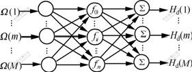
Fig. 1 Schematic diagram of neural networks architecture
Let
C1=[fT(¦ё(1)); fT(¦ё(2)); Ў; fT(¦ё(M))]T (10)
then Eqn.(8) can be rewritten as
 (11)
(11)
Define error function as
e=Md-Hd (12)
and performance index V as
 (13)
(13)
then the steepest descent algorithm for the approximate square error is
W(k+1)=W(k)+¦ЗC1e (14)
where ¦З is the learning rate. Obviously, besides W the coefficients of a linear phase FIR filter can also be obtained by using Eqn.(14). So we can design a linear phase FIR filter by training the amplitude response of a desired filter based on the neural networks algorithm.
It is necessary to study the convergence and stability of the neural networks algorithm.
Convergence Theorem 1 when learning rate ¦З satisfies 0Јј¦ЗЈј2/(n+1), the neural networks algorithm is convergent, where n+1 is the number of hidden nodes of the neural networks.
 Proof Define Eqn.(13) as a Lyapunov function, then
 (15)
(15)
Because

 (16)
(16)
where  is the square of Euclidean norm. Therefore, Eqn.(15) can be expressed as

 (17)
(17)
Because ¦ЗЈѕ0, it is easy to see that if 0Јј¦ЗЈј  , then ¦¤V(e)Јј0, and the algorithm is convergence. Because
 (18)
(18)
then
 (19)
(19)
According to Eqns.(8), (9) and (10), we have 1ЎЬ  ЎЬn+1. Hence the neural networks algorithm is convergent if 0Јј¦ЗЈј2/(n+1). This completes the proof.
It is easy to see that the Lyapunov function V(e) is a positive definite from Eqn.(13). When 0Јј¦ЗЈј2/(n+1),
 (20)
(20)
thus ¦¤V(e)/¦¤k is negative definite. Therefore, the origin (e=0) is asymptotically stable.
The neural networks algorithm is summarized as follows:
Step 1 Sample uniformly the desired amplitude response Md(¦ё) in ¦ёЎК[0, ¦Р] to get its discrete matrix Md, and use the discrete matrix as a set of training samples. Next produce randomly initial weight matrix W. Then define an arbitrary small positive real number ¦Е, and let 0Јј¦ЗЈј2/(n+1).
Step 2 Produce new predicted output Hd of neural network using Eqn.(11).
Step 3 Calculate e and V(e) via Eqns.(12) and (13).
Step 4 Update the weight matrix W using back- propagation algorithm according to Eqn.(14).
Step 5 if V(e)Јѕ¦Е, go to step 2, otherwise, close the training of the neural network.
3.2 Design example
In this section, two simulation examples will be given. The purpose is to verify the convergence theorem of the proposed neural network algorithm and to support the optimal design approach of FIR filters.
Example 1 Considering the example 1 in Ref.[14], design an 80th-order FIR notch filter specified by ¦ёm=0.35¦Р.
Let N=81, ¦Е=10-10, ¦З=0.024 4, and M=41. In order to prevent ripple and pulse in pass-band, define two samples in transition bands that their amplitude values are 0.78 and 0.25, respectively. After 21 times training, the algorithm converges to a FIR notch filter with the amplitude response as shown in Fig.2. The actual notch filter parameters are ¦ёm=0.349 9¦Р and ¦¤¦ё=0.092 4¦Р for a=-3.010 3 dB. Comparing with the design example 1 in Ref.[14], the actual 89th-order filter parameters are ¦ёm=0.349 8¦Р and ¦¤¦ё=0.149 6¦Р for amplitude attenuation a=-3.010 3 dB using analytical design algorithm.
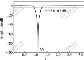
Fig.2 Amplitude response for example 1
Example 2 Consider a 2 000th-order multi-band- pass FIR linear-phase filter design example:
H(¦ё)=0 for 0ЎЬ¦ёЎЬ0.15¦Р, 0.29¦РЎЬ¦ёЎЬ0.43¦Р, 0.57¦РЎЬ¦ёЎЬ0.71¦Р, 0.85¦РЎЬ¦ёЎЬ¦Р
H(¦ё)=1 for others.
Let N=2 001, ¦Е=10-20, ¦З=9.99ЎБ10-4, and M=1 001. As in example 1, define two samples in every transition band that their amplitude values are 0.25 and 0.78, respectively. It takes the proposed algorithm 42 times training to converge to a FIR filter with the minimum stop-band attenuation 80 dB. The amplitude response of the FIR filter is shown in Fig.3.
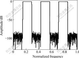
Fig.3 Amplitude response for example 2
4 Optimal design of typeўтFIR filters
4.1 Algorithm description
The neural networks architecture is as same as Fig.1, and the activation function of ith hidden neuron is
fi=cos[(i-0.5)¦ё(m)] (i=1, Ў, n) (21)
Let
C2=[fT(¦ё(1)); fT(¦ё(2)); Ў; fT(¦ё(M))]T (22)
then Eqn.(8) can be rewritten as
 (23)
(23)
Now we define error function and performance index V as Eqns.(11) and (12), respectively, then the steepest descent algorithm for the approximate square error is
W(k+1)=W(k)+¦ЗC2e (24)
where ¦З is the learning rate. Then the convergence theorem of the algorithm can be described as follows.
Convergence Theorem 2 When learning rate ¦З satisfies 0Јј¦ЗЈј2/n, the algorithm of the neural network is convergent, where n is the number of hidden nodes of the neural networks.
The proof process and the calculating steps of the weight vector W are same as those described in subsection 3.1.
4.2 Design example
Example 3 Considering example 1 in Ref.[15], we design a 77th-order linear-phase low-pass FIR filter with pass-band of [0, 0.4¦Р] and stop-band of [0.45¦Р, ¦Р].
Let N=78, ¦Е=10-5, ¦З=0.025 64, and M=40. It takes the proposed algorithm 12 times training to converge to a FIR filter with the amplitude response as shown in Fig.4. We can see that the ripple of the designed filter in low-pass band and high-stop band is as same as that of the designed 78th-order filter based on a multiple exchange algorithm in Ref.[15].
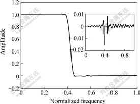
Fig.4 Amplitude response and associated error for example 3
5 Optimal design of type ўу FIR filters
5.1 Algorithm description
The neural networks architecture has shown in Fig.1, and the activation function of ith hidden neuron is
fi=sin[i¦ё(m)] (i=1, Ў, n) (25)
Let
C3=[fT(¦ё(1)); fT(¦ё(2)); Ў; fT(¦ё(M))]T (26)
then Eqn.(8) can be rewritten as
 (27)
(27)
Similarly, we define error function and performance index V as Eqns.(11) and (12), respectively, then the steepest descent algorithm for the approximate square error is
W(k+1)=W(k)+¦ЗC3e (28)
Convergence Theorem 3 When learning rate ¦З satisfies 0Јј¦ЗЈј4/(n+1), the algorithm of the neural network is convergent, where n is the number of hidden nodes of the neural networks.
5.2 Design example
Example 4 Considering example 2 in Ref.[15], we design a 78th-order linear-phase digital differentiator with low-pass frequency response. The low-pass differentiator has ideal frequency response j¦ё on lower frequency band and null frequency response on higher frequency band. The lower band edge of 0.8¦Р and higher edge of 0.85¦Р are used in this example.
Let N=79, ¦Е=10-10, ¦З=0.05, and M=40. After 5 times training, the algorithm converges to the low-pass differentiator with the amplitude response and associated error as shown in Fig.5. It can be seen that the ripple of the designed filter in low-pass band and high-stop band is less than 0.015. Comparing with the design example 2 in Ref.[15], the ripple of the designed 78-order filter in low-pass band and high-stop band is bigger than 0.02 based on a multiple exchange algorithm.
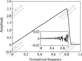
Fig. 5 Amplitude response and associated error for example 4
Example 5 Design a 78th-order digital Hilbert transformer. The Hilbert transformer has ideal frequency response ЁCjexp(-j¦Б¦ё) for 0Јј¦ёЈј¦Р and jexp(-j¦Б¦ё) for -¦РЈј¦ёЈј0.
Let N=79, ¦Е=10-10, ¦З=0.005, and M=40. Let the initial weights be random, and define two samples in the transition band that their amplitude values are -0.35 and -0.80, respectively. After 5 times training, the algorithm converged to a Hilbert transformer with the amplitude response and associated error as shown in Fig.6.
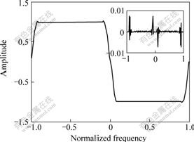
Fig.6 Amplitude response and associated error for example 5
6 Optimal design of type ўф FIR filters
6.1 Algorithm description
The architecture of neural networks is also as same as Fig.1, and the activation function of ith hidden neuron is
fi=sin[(i-0.5)¦ё(m)] (i=1, Ў, n; n=N/2) (29)
Let
C4=[fT(¦ё(1)); fT(¦ё(2)); Ў; fT(¦ё(M))]T (30)
then Eqn.(8) can be rewritten as
 (31)
(31)
In the same way, we define error function and performance index V as Eqns.(11) and (12), respectively, then the steepest descent algorithm for the approximate square error is
W(k+1)=W(k)+¦ЗC4e (32)
where ¦З is the learning rate. The convergence theorem of the algorithm can be described as follows.
Convergence Theorem 4 When learning rate ¦З satisfies  , the algorithm of the neural network is convergent, where n is the number of hidden nodes of the neural networks.
6.2 Design example
Example 6 Design a 79th-order linear phase FIR narrow band-pass filter specified by ¦ёm=0.35¦Р.
Let N=80, ¦Е=10-5, ¦З=0.025 64, and M=41. After 13 times training, the algorithm converged to an FIR filter with the amplitude response as shown in Fig.7. The actual filter parameters are ¦ёm=0.350 0¦Р and ¦¤¦ё= 0.058 0 ¦Р for a=-6.020 6 dB.
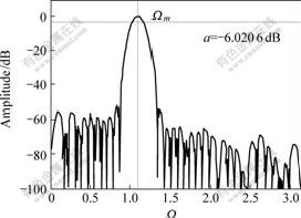
Fig. 7 Amplitude response for Example 6
7 Conclusions
1) Four optimal methods for designing FIR linear phase digital filters based on neural network algorithms are presented. Their main idea is to minimize the frequency-domain error function. Because of being not involved in matrix inverse operations, these methods solve the difficult problem effectively on designing high order FIR filters. The ripples in pass-bands are less than 0.1 decibels, the attenuations in stop-bands are more than sixty decibels, and the border frequencies of pass-bands and stop-bands are easily controlled precisely.
2) The first method can design a linear-phase FIR digital filter (LPFIRDF) with arbitrary amplitude frequency response, but the second approach can only design a class of LPFIRDF with magnitude value 0 on ¦ё=¦Р (such as a low-pass or band-pass LPFIRDF), the third method can merely design a class of LPFIRDF with magnitude value 0 on ¦ё=0 and ¦ё=¦Р (such as a band-pass or multi-band-pass LPFIRDF), and the fourth approach can only design a class of LPFIRDF with magnitude value 0 on ¦ё=0 (such as a high-pass or band-pass LPFIRDF).
References
[1] HE Yi-gang, JIANG Jing-guang, WU Jie, et al. Universal active currentЁCmode filter[J]. Acta Electronica Sinica, 1999, 27(11): 21-23.(in Chinese)
[2] HE Yi-gang, JIANG Jing-guang, WU Jie. Fully differential 4th-order bessel filter accurately designed with group delay[J]. Acta Electronical Sinica, 2002, 30(2): 249-251.(in Chinese)
[3] CHENG Jiang, HE Yi-gang. A Fully balanced two-input high frequency widely linear tunable OTA and its application to filters[J]. Journal of Circuits and Systems, 2004, 9(4): 50-53.(in Chinese)
[4] HE Yi-gang, SUN Yi-chuang. A neural-based nonlinear L1ЁCnorm optimization approach for fault diagnosis of nonlinear circuits with tolerance[J]. IEE Proceedings Circuits Devices and Systems, 2001, 148(4): 223-228.
[5] HE Yi-gang, TAN Yan-hong, SUN Yi-chuang. Wavelet neural network approach for fault diagnosis of analog circuits[J]. IEE Proceedings Circuits Devices and Systems, 2004, 151(4): 379-384.
[6] CHEN C K, LEE J H. Design of digital all-pass filters using a weighted least squares approach[J]. IEEE Transactions on Circuits and Systems II, 1994, 41(5): 943-953.
[7] LIM Y C, LEE J H, CHEN C K, et al. A weight least squares algorithm for quasiЁCEquiripple FIR and IIR digital filter design[J]. IEEE Transactions on Signal Processing, 1992, 39(3): 551-558.
[8] LEE J H, CHEN C K, LIM Y C. Design of discrete coefficient FIR digital filters with arbitrary amplitude and phase responses[J]. IEEE Transactions on Circuits and Systems II, 1993, 40(7): 444-448.
[9] LAI Xiao-ping. A random sampling recursive leastЁCsquares approach to the design of FIR digital filters[J]. Journal of Signal Processing, 1999, 15(3): 260-264. (in Chinese)
[10] LU Wu-sheng. A unified approach for the design of 2-D digital filters via semidefinite programming[J]. IEEE Transactions on Circuits and Systems I, 2002, 49(6): 814-825.
[11] TUAN H D, SON T T, TUY H, et al. New linear-programming-based filter design[J]. IEEE Transactions on Circuits and Systems II, 2005, 52(5): 276-281.
[12] ZHAO Hui, YU Jue-bang. A novel neural networkЁCbased approach for designing 2-D FIR filters[J]. IEEE Transactions on Circuits and Systems II, 1997, 44(11): 1095-1099.
[13] WANG Yan, LIAO Xiao-feng, YU Jue-bang. Complex neural network on designing FIR digital filter[J]. Journal of Signal Processing, 1999, 15(3): 193-198.(in Chinese)
[14] PAVEL Z, MIROSLAV V. Fast analytical design algorithms for FIR notch filters[J]. IEEE Transactions on Circuits and Systems I, 2004, 51(3): 608-623.
[15] PEI Soo-chang, WANG Peng-hua. Design of equiripple FIR filters with constraint using a multiple exchange algorithm[J]. IEEE Transactions on Circuits and Systems I, 2002, 49(1): 113-116.
(Edited by YANG You-ping)
Foundation item: Project (50677014) supported by the National Natural Science Foundation of China; project (20060532002) supported by the Doctoral Special Fund of Ministry of Education, China; project (NCET-04-0767) supported by the Program for New Century Excellent Talents in University; projects(06JJ2024, 03GKY3115, 04FJ2003, and 05GK2005) supported by the Foundation of Hunan Provincial Science and Technology
Received date: 2006-05-09; Accepted date: 2006-07-16
Corresponding author: HE Yi-gang, Professor; Tel: +86-731-8822224; E-mail: yghe@hnu. cn

