J. Cent. South Univ. Technol. (2010) 17: 1251-1257

DOI: 10.1007/s11771-010-0628-8

Improvement of prediction model for work roll thermal contour in hot strip mill

WANG Lian-sheng(王连生), YANG Quan(杨荃), HE An-rui(何安瑞),

ZHENG Xuan(郑宣), YU Hong-rui(于洪瑞)

National Engineering Research Center for Advanced Rolling Technology,

University of Science and Technology Beijing, Beijing 100083, China

? Central South University Press and Springer-Verlag Berlin Heidelberg 2010

Abstract: Though high accuracy of the thermal contour was obtained while adopting finite element method, it could not meet the real-time requirement. One-dimensional finite difference method could realize real-time control in the case of neglecting both the circumferential and radical heat exchange, but the over-simplified modes resulted in poor accuracy. And two-dimensional full explicit difference was also limited in practical application since its time step was restricted to keep the model stable. Consequently, a new method of alternating direction finite difference was introduced and discussed in the model’s stability, calculating speed and  precision. Specific work roll after one real rolling unit was researched, The result shows that error of temperature on work roll surface between measured and calculated values is within 5 ℃. The influence of rolling rhythm and strip width on thermal crown was also studied. The conclusion is verified theoretically and practically that it can maintain absolutely stable and meet the online requirement.

Key words: hot rolling; finite element; finite difference; work roll; thermal contour

1 Introduction

In hot strip rolling, thermal contour being one of most significant mill disturbance affects product quality of strip gauge, crown, and shape. Much attention was paid to this typical heat transfer program in rolling mills. To predict the work roll thermal contour precisely was always one difficult aspect in shape control. The calculation of thermal contour was based on that of temperature field in work roll [1-2]. Usually, two methods are used to calculate the temperature field, such as finite element method (FEM) and finite difference method. Most of researchers adopted finite difference method [3-5], for one-dimensional (1-D) finite method, the roll was considered as a series of circular discs, and there were no temperature gradients within a disc. Hence, the surface temperature, the core temperature and the bulk temperature were identical in each disc. The thermal profile could be easily calculated by multiplying the thermal expansion coefficient and the temperature difference between discs. The 1-D solution took a shorter time, but the radial temperature gradient was neglected. Currently, the 1-D method, however, though presented in simple equations, was able to meet the application accuracy, so it was widely used in hot strip rolling [6-7]. A simplified FEM was used to analyze the temperature field and thermal contour of roll [8], and the corresponding models were built according to the practical boundary conditions. Transient roll temperature field and thermal contour were simulated by ANSYS FEM software with considering transient thermal contact and complex boundary condition. The thermal contour results of roll obtained by FEM simulation were in good agreement with the measured data, indicating that simplified FEM models and results were correct. However, FEM method was time-consuming, which was limited to its practical application.

In this work, according to the characteristics of thermal contour, alternating direction finite difference was applied to solving the temperature field and then calculating the thermal contour. On the premise of calculation precise, the problem was simplified, which met the production requirement. Alternating direction finite difference adopted the implicit difference during the first half time step in x direction while the explicit difference did in y direction. When in the second half time step, the sequence was exactly reversed (implicit difference in y direction and the explicit difference in x direction).

2 Calculation of work roll temperature field and thermal contour model

In hot strip rolling, the behaviors of heat exchange are so complex that it is almost impossible to describe them exactly quantitatively. Therefore, it is necessary to simplify or sometimes even neglect the heat exchange that slightly affects work roll temperature field in practical application. ZHANG et al [3] studied the work roll temperature field and thermal profile in hot strip mills, and the results indicated that work roll temperature came from two aspects: the basic temperature that was the average temperature of work roll and the periodical temperature that only existed on the roll surface. STEVVENS [9] measured the work roll temperature in rough rolling mill and noticed that the temperature varied dramatically and periodically within the depth of 2-3 mm in roll surface whereas more than 99% of the inner part of work roll had the symmetric temperature distribution. As high-speed of roll rotation, the fluctuation of temperature field was limited to happen on extreme thin surface. Thus, the thermal conductivity along with the circumferential direction could be ignored and only the thermal conductivity in the direction of diameter and axis was taken into account, which enabled the three-dimensional temperature field problem to be simplified into a two-dimensional symmetric one.

2.1 Equation of heat conductivity and difference

The first step was to assume that roll material was isotropic, no inner heat source existed, the initiative temperature was 40 ℃, the roll was divided into various types of elements, and each type needed the differential equation [10-13]. In the cylindrical coordinate system, the heat conductivity was simplified as the following equation:

                (1)

where r is the material density; c_p is the material specific heat capacity; k is the thermal conductivity; T is the temperature; r is the radial coordinate; and x is the axial coordinate.

The division model of work roll temperature field is illustrated in Fig.1, where L_w is the length of the work roll, B is the width of strip, L₁ is the length of contact part with bearing, L₂ is the length of transition part of roll, and L₃ is the length of non-contact part with strip at each side. According to the actual situation, the axial thickness of cell at neck was larger than that at body and the radial thickness of each body cell increased at the rate of 1.2 times from outside to inside.

When calculating the element temperature, there were several heat convection sections between strip and roll, roll and air, roll and cooling water, elements as well. The grid points of the work roll had various types of heat transfer. There were five types of differential equations obtained by using energy conversation law. The first type of differential equation was internal grid points, the second type was surface of the roll grid points, the third one was side of the roll grid points, the fourth one was the corner grid points and the last one was axis grid points.

The energy relationship between internal grids is shown in Fig.2, and other relationships are similar.

The differential equations of the grids in the five different sections were described as follows in the first half and the second half time steps separately.

The differential equations of internal grid points were:

 (2)

=

                         (3)

Fig.1 Dividing up temperature field model of work roll: ①—Heat exchange surface of roll and bearing part; ②—Heat exchange surface between roll and air; ③—Heat exchange surface between roll and cooling water in rolling and water cooling process or surface between roll and air in air cooling process; ④—Heat exchange surface between roll and strip in rolling process

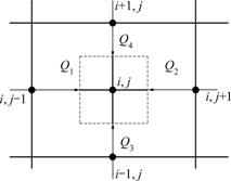
Fig.2 Energy relationship chart between internal grids

The differential equations of core grid points were:

                    (4)

            (5)

The differential equations of surface grid points were:

           (6)

     (7)

The differential equations of left side grid points were:

(8)

         (9)

The differential equations of right side grid points were:

            (10)

                  (11)

The differential equations of left corner grid points were:

    (12)

(13)

The differential equations of right corner grid points were:

=

  (14)

(15)

where

  

  

 stands for the temperature of unit (i, j) at the time step of n+1/2; Dt is the time step; Dx is the axial space step; Dr is the radial space step; h is the coefficient of equivalent heat exchange between work roll and the one among bearings, air, cooling water and strip; and T_out is the outside medium temperature of strip, air or water while heat exchange differs.

 

2.2 Compution speed and stability

Solving alternating direction finite difference equations was essentially identical to solving a number of tridiagonal equations and the solving form was as the following equation:

     (16)

where N_r and N_x are the radial and axial units; and a, b, c and d are the equation coefficients.

For an n-order tridiagonal equation, the catch-up algorithm could solve it quickly. Specifically, to calculate the work roll temperature, the right side vector of the equations should be solved at each time before solving tridiagonal linear equations and the calculating times were approximately 3n. A tridiagonal equation needs to be calculated 8n times when alternating direction finite difference method was used. For explicit finite difference method, it was 5n times. When considering at each time step, the axial implicit and radial explicit calculations were carried out in each step, thus the total time would be (2×8n)/(5n)=3.2 times than time calculating completely explicit difference method. Obviously, both methods were at the same order of magnitude and met the practical requirements.

The convergence and stability had the most priority when judging whether any type of difference equations could be applied in practice. It proved that the alternating direction finite difference method could meet the requirements. The inequality for the stability condition of two-dimension complete difference equation was shown as follows:

≥0                 (17)

For the complete explicit difference equation, it should be limited by the inequality (17) to maintain stable. But the alternating difference equation had no such limits. As a result, it was accessible to increase the time step for reducing computing time as long as the accuracy was acquired or to decrease space step for raising the accuracy, which demonstrated the merits of the alternating difference equation.

2.3 Calculation of thermal contour

Based on calculation of the temperature field of work roll, thermal contour was obtained. So as soon as the temperature distribution was known, the roll thermal expansion along the diameter was calculated by the following equation.

        (18)

where u is the amount of thermal expansion; n is the Poisson ratio; b is the linear thermal expansion coefficient of the material; R is the radius of the work roll and T₀ is the initial temperature (40 ℃).

After calculating the relative values of diameter expansion at different points of work roll, the thermal contour was gained and then the expansion deviation between the center and edge, which was the thermal crown, could be acquired.

3 Optimization of work roll heat transfer coefficient

3.1 Objective function proposed to optimize

In rolling process, the assumed boundary conditions had large effects on temperature distribution. The work roll condition consisted of three parts: rolling, water cooling and air cooling. The boundary condition of work roll could be divided into four kinds of heat transfers between work roll and strip as well as cooling water, air and bearings [14-16].

                 (19)

                             (20)

              (21)

                                                       (22)

where q_s, q_rad and q_w represent heat flux densities of strip contact area, radiation and water cooling district, respectively; l_s, l_rad and l_w represent the arc lengths indicating the work roll and strip contacting, radiation section and water cooling section, respectively; T_r, T_s and T_w are the temperatures of work roll, strip and cooling water, respectively; h_s, h_w and h_air represent the coefficients of convection between work roll and strip, work roll and cooling water, work roll and air, respectively; e and d are the strip thermal radiation rate and thermal radiation constant, respectively.

In practical production, the right parameters of model directly determine whether the model could be applied accurately. As data indicated that h_s was a function relevant to parameters of R, P, B, T_s, and Dh, which orderly represented radius of work roll, rolling force, the width of strip, the temperature of strip and the reduction respectively. h_w was a function relevant to parameters of h_Q and h_P in which h_Q represented the relative value of cooling water coefficient that was related to watering density and h_P was the relative value of cooling water coefficient that was related to watering pressure. To meet the continuously variable surrounding requirements, the correction factor of the model must be introduced.

                      (23)

                               (24)

The parameters of k_s, k_w and h_air should be specified to determine the heat transfer coefficient between work roll and surroundings and the vector K=[k_s, k_w, h_air] was used in following calculation. The data about the temperature distribution  of work roll surface at a specific time after rolling m units was measured and the same distribution from models was collected. The aim was to find a vector K=[k_s, k_w, h_air] that minimized the deviation between the measured and calculated temperature distribution, so the target function was detailed as follows:

          (25)

where DT is the target function; m is the number of rolling units; n is the sample points in each rolling unit; T_i(j) is the j point of the i rolling unit; is the actual temperature value of the j point of the i rolling unit; p_ms stands for the assumed parameters related to the rolling units; K is the vector (K=[k_s, k_w, h_air]). The target is to minimize the g function by searching for the corresponding value of K.

3.2 Heat transfer coefficient optimization

Genetic algorithm derived from the natural selection and group evolutionary mechanism was a global optimization algorithm. Compared with other methods like traditional gradient, Newton and variable scale method, genetic algorithm (GA) coded the optimization factors instead of the coefficient itself. Additionally, the algorithm was a parallel operation to the groups, which to a large extent results in the global optimal solution. The operation was random, not following any determinate principles. Due to the heuristic search, it characterized itself with high efficiency. The genetic algorithm had no specific limits on the complexity of functions and had the global optimization ability, so it was selected to solve the coefficient optimization of work roll temperature field model. On the basis of practical data, more reasonable parameters of model were obtained by off-line GA optimization.

3.2.1 Optimization steps

(1) Coding. Real number was used to code. The group size P_op was 30, the evolution generation N was 100, intercross probability p_c was 0.85 and variation probability p_m was 0.1. According to experience, the range of variables k_s was set in [0, 5], k_w in [0.1, 2.5] and h_air in [20, 300].

(2) Fitness calculation. Choose five points as reference, which were the axial middle points of work roll, drive and work side surface marking points and two quartered points. The modified target function was as follows:

                  (26)

DT was required to become zero, so the fitness function F_t was

                           (27)

(3) Group selection. Using the roulette method, the chromosome chosen probability was in direct proportion to the new fitness value, which ensured the excellent chromosome to get the evolution chance.

(4) Intercross. In this method, real number was used to code. The length of chromosome was 3 and single copulation bit intercross method was used. The bit was generated at random and made arithmetic intercross of right chromosome. The arithmetic intercross was that the genes from two parent chromosomes generate child chromosomes by the following method.

           (28)

where x₁ and x₂ are the two parent chromosomes; and  are the child chromosomes; and r∈(0, 1) is a random value.

(5) Mutation. Inhomogeneous variation method was selected. To a specific parent v, if its element x_k was chosen to mutate, the child  was generated, where  varied randomly as follows:

   (29)

 and  are the upper and lower bounds of x_k. Function Δ(g, y) gave a value within [0, y], and Δ(g, y) tended to be zero with the increment of g. The frame is shown in Fig.3.

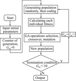
Fig.3 Flow chart of GA

3.2.2 Optimized output from genetic algorithm

After the generations of 100, the target value came to be stable when the generation is 89. The result shows that DT is 1.956 ℃ in Fig.4.

4 Model verification

Taking the hot rolling production line of a domestic iron and steel company for the target to study, the model established above was applied to calculating the temperature distribution on the surface of work roll after one rolling unit including the number of 120 strips with the width of 1.05, 1.27 and 1.50 m. As soon as the rolling process was over, the roller was cooled by water for    5 min and by air for 10 min. The surface temperature of work roll was measured at each 100 mm position. As seen from Fig.5, when the time cooled by water t_w is 1, 2 and 5 min the surface temperature is simulated. The result shows that the center point temperature along with axial direction is reduced from 50.2 and 45.6 to 41.1 ℃. Meanwhile, the temperature curve changes after 5 min and becomes more “round”. Compared the measured data of t_w=5 min and the time cooled by air t_a=10 min with the calculated value, the surface temperature distribution indicates that the new model reaches good agreement with the measured data in tendency of the curve and the maximum deviation of temperature between measured data and the new model is less than  5 ℃. The center temperature becomes 54.2 ℃ from 41.1 ℃ after 10 min air cooling because the energy of inner grid points gradually transfers heat to the surface ones while the energy of air to surface grid points is less than that of inner grid points. At this time, the temperature curve does not remain uniform, but seems “C” shape.

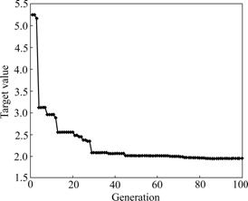
Fig.4 Evolution curve of target value

Fig.5 Comparison of work roll temperature after rolling

Taking two kinds of real rolling units to calculate, the interval time t_I are 50 and 36 s, respectively. The temperature of strip is 980 ℃, the reduction is 11 mm, rolling force is 16 MN, the rolling shift is 0 mm, the thermal conductivity is 38 W/(m·K), specific heat capacity is 470 J/(kg·K), the cooling water temperature is 33 ℃, the diameter of work roll is 780 mm, and the density of the work roll material is 7 850 kg/m³. The rolling rhythm R_h is defined by

×100%                         (30)

where t_R is the rolling time.

The impact of rolling rhythm on the thermal is illustrated in Fig.6.

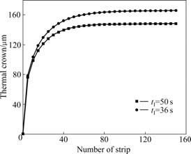
Fig.6 Work roll thermal contour variation due to rolling rhythm when t_R=50 s

At the stable stage of rolling, the gap of thermal contour between two rolling units reaches 18 μm. In this situation, the thermal equilibrium of work roll is attained after rolling 50 strips and at this time the thermal contour becomes stable.

Taking rolling time t_R=50 s as a constant, interval time t_I=50 s, thermal crown data are shown in Fig.7. It shows the result of lumped case. There are two thermal crown jumps after #3 and #4 coils due to the width drop while keeping other parameters unchanged, such as reduction. Because with the increase of strip width, strip needs to share energy with the surface of work roll so that the relative expansion along with the radical direction must be reduced. Similarly, after the rolling time of #8 coil the change of thermal crown is small while width increases. Note that thermal crown distribution with one process (idling and rolling) is nearly linear though the solution equation shows that the result should be curve. Note that after 10 coils the thermal crown is 98 μm and the roll still does not reach stable stage.

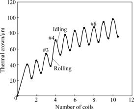
Fig.7 Variation of work roll thermal contour with numbers of rolled strip

5 Conclusions

(1) The calculation accuracy is improved while the radical heat transfer is not considered by one dimensional method and the curve tendency reaches good agreement with measured value.

(2) The absolute stability is gained in comparison with the explicit difference method and the relative space step is allowed when the time step is small if the accuracy is met. The calculation speed that can meet strip shape control requirement is verified.

(3) Heat transfer coefficients optimization of work roll is conducted by introducing genetic algorithm and its effectiveness is verified by practical results.

(4) The impact from rolling rhythm on the thermal contour is simulated and the result shows that after 50 strips the thermal contour reaches a stable stage, which is in line with the practical situation.

References

[1] GINZBURGVB. Application of coolflex model for analysis of work roll thermal conditions in hot strip mills [J]. Iron and Steel Engineer, 1997, 11: 42.

[2] GINZBURGVB,GIUSTO D. Roll thermal crown (RTC) control system [J]. MPT Metallurgical Plant and Technology International, 1994, 17(4): 80-81.

[3] ZHANG Xun-li, ZHANG Jie, WEI Gang-cheng, MA Shao-hua. Study on work roll temperature field and thermal profile in hot strip mills [J]. Metallurgical Equipment, 2002, 6(1): 133-136. (in Chinese)

[4] WANG Ren-zhong, HE An-rui, YANG Quan. Thermal contour model of work rolls in hot wide strip mills [J]. Journal of University of Science and Technology Beijing, 2004, 26(6): 654-657. (in Chinese)

[5] WANG Xiao-dong, YANG Quan, HE An-rui, WANG Ren-zhong. Comprehensive contour prediction model of work roll used in online strip shape control model during hot rolling [J]. Ironmaking and steelmaking, 2007, 34(4): 303-311.

[6] PANJKOVIC V, FRASER G, YUEN D. Applications of the crown and shape model in blue scope steel’s western por hot strip mill [J]. Iron and Steel Technology, 2004, 1(10): 98-107.

[7] CAMPOS A M, GARCI D F, ABAJO N. Real-time rule based control of the thermal crown of work rolls installed in hot strip mills [J]. IEEE Transactions on Industry Applications, 2004, 40(2): 642-649.

[8] GUO Zhong-feng, LI Chang-sheng, XU Jian-zhong, LIU Xiang-hua. Analysis of temperature field and thermal crown of roll during hot rolling by simplified FEM [J]. Journal of Iron and Steel Research International, 2006, 13(6): 27-30.

[9] STEVENS P G. Increasing work-roll life by improved rolling practice [J]. J Iron and Steel Inst, 1971(1): 1-6.

[10] TSENG A A, TONG S X, CHEN T C. Thermal expansion and crown evaluations in rolling processes [J]. Material and Design, 1996, 1(4): 193-204.

[11] TOPNO R, PRAKASH K, JHA S K. Different colling of hot rolled angles to reduce thermal camber [J]. Steel Times International, 2003, 27(4): 18-20.

[12] COLAS R. Modeling heat transfer during hot rolling of steel strip model [J]. Simul Mater Sci Eng, 1995, 3(4): 437-453.

[13] PLLONE G T. Transient temperature distribution in work rolls during hot rolling of sheet strip [J]. Iron Steel Eng, 1983, 5(12): 21-24.

[14] YUEN W Y D. Research on the steady-state temperature distribution in a rotating cylinder subject to heating and cooling over its surface [J]. Trans ASME, 1984, 106(8): 578-583.

[15] SUMI H. A numerical model and control of plate crown in the hot strip or plate rolling [J]. Advanced Technology of Plasticity, 1984, 1(2): 1360-1365.

[16] HOGSHEAD T H. Temperature distributions in the rolling of metal strip [D]. Pennsylvania: Camegie Mellon University, 1988.

(Edited by YANG You-ping)

Foundation item: Project(2006BAE03A13) supported by the National Science and Technology Support Program during the 11th Five-Year Plan Period

Received date: 2009-12-29; Accepted date: 2010-03-11

Corresponding author: WANG Lian-sheng, PhD, Professor; Tel: +86-10-62332598-6310; E-mail: wangliansheng2002@sina.com